深度学习
深度学习
常见深度学习模型
- 卷积神经网络(Convolutional Neural Networks,CNN)
- 主要用于图像处理,如图像分类、目标检测、图像分割等
- 特点是使用卷积层来自动提取图像的局部特征,并通过池化层减少参数数量,提高计算效率
- 循环神经网络(Recurrent Neural Networks,RNN)
- 适用于处理序列数据,例如自然语言处理(NLP)、语音识别等
- 自编码器(Autoencoders)
- 一种无监督学习模型,通常用于降维、特征学习或者异常检测
- 生成对抗网络(Generative Adversarial Networks,GAN)
- 包含生成器和判别器,生成器负责创建看起来真实的假样本,判别器负责区分真假
- 广泛用于图像合成、视频生成领域
- Transformer
- 主要用于自然语言处理任务
- 深度强化学习(Deep Reinforcement Learning,DRL)
- 图神经网络(GNN,Graph Neural Network)
Pytorch
PyTorch 是一个开源的深度学习框架,主要用于构建、训练和部署神经网络模型。
安装
- 创建新的anaconda环境:
conda create -n 环境名 python=版本 - 切换环境:
conda activate 环境名 - 安装Pytorch:
pip install torch - 安装NumPy:
pip install numpy(不安装使用torch时会有警告)
Tensor张量
pytorch中的数据结构,类似于NumPy的ndarray,并支持GPU加速
可看做是多维数组 + 能自动求导
创建Tensor的方式
直接创建
data: 数据, dtype: 可指定元素类型,默认float32
torch.tensor(data, dtpye):创建Tensor的函数(推荐用这个)
1
2
3
4
# 创建一维的标量
t1 = torch.tensor(10)
print(f't1: {t1}, type: {type(t1)}')
# t1: 10, type: <class 'torch.Tensor'>使用python数组创建
1
2
3
4
5
arr = [[1, 2], [3, 4]]
t2 = torch.tensor(arr)
print(f't2: {t2}, type: {type(t2)}')
# t2: tensor([[1, 2],
# [3, 4]]), type: <class 'torch.Tensor'>使用numpy的ndarray创建
1
2
3
4
5
6
data = np.array([[1, 2], [3, 4], [5, 6]])
t3 = torch.tensor(data)
print(f't3: {t3}, type: {type(t3)}')
# t3: tensor([[1, 2],
# [3, 4],
# [5, 6]]), type: <class 'torch.Tensor'>torch.Tensor()方式torch.Tensor():Tensor的构造函数
1
2
3
4
5
# 创建2行3列的Tensor
t4 = torch.Tensor(2, 3)
print(f't4: {t4}, type: {type(t4)}')
# t4: tensor([[2.3420e+18, 1.8581e-42, 0.0000e+00],
# [0.0000e+00, 0.0000e+00, 0.0000e+00]]), type: <class 'torch.Tensor'>创建线性张量
1
2
3
4
5
6
7
8
9
# 指定范围,左闭右开
t1 = torch.arange(0, 10, 2)
print(f't1: {t1}, type: {type(t1)}')
# t1: tensor([0, 2, 4, 6, 8]), type: <class 'torch.Tensor'>
# 等差数列
t2 = torch.linspace(0, 10, 4)
print(f't2: {t2}, type: {type(t2)}')
# t2: tensor([ 0.0000, 3.3333, 6.6667, 10.0000]), type: <class 'torch.Tensor'>创建随机值的张量
1
2
3
4
5
6
7
8
9
10
11
12
13
14
15
16
17
18
19
20
21
# 设置随机种子,默认采用当前时间戳
# torch.initial_seed()
# 设置随机种子,可手动指定值
torch.manual_seed(3)
# 创建随机张量,符合均匀分布
t1 = torch.rand(size=(2, 3))
print(f't1: {t1}, type: {type(t1)}')
# t1: tensor([[0.6203, 0.8253, 0.1595],
# [0.6263, 0.2207, 0.9387]]), type: <class 'torch.Tensor'>
# 创建随机张量,符合正态分布
t2 = torch.randn(size=(2, 3))
print(f't2: {t2}, type: {type(t2)}')
# t2: tensor([[ 0.7625, 1.4948, -0.5175],
# [-0.4186, -0.9309, 0.4139]]), type: <class 'torch.Tensor'>
# 创建随机张量,都是整数
t3 = torch.randint(low=0, high=2, size=(2, 3))
print(f't3: {t3}, type: {type(t3)}')创建有指定值的张量
1
2
3
4
5
6
7
8
9
10
11
12
13
14
15
16
17
18
19
20
21
22
23
24
25
# 创建全是1的张量
t1 = torch.ones(2, 3)
print(f't1: {t1}, type: {type(t1)}')
# t1: tensor([[1., 1., 1.],
# [1., 1., 1.]]), type: <class 'torch.Tensor'>
# 根据已有张量,创建size一样的全1张量
t2 = torch.tensor([[1, 2], [3, 4], [5, 6]])
t3 = torch.ones_like(t2)
print(f't3: {t3}, type: {type(t3)}')
# t3: tensor([[1, 1],
# [1, 1],
# [1, 1]]), type: <class 'torch.Tensor'>
# 创建全是0的张量
t4 = torch.zeros(2, 3)
print(f't4: {t4}, type: {type(t4)}')
# t4: tensor([[0., 0., 0.],
# [0., 0., 0.]]), type: <class 'torch.Tensor'>
# 创建全是指定值的张量
t5 = torch.full(size=(2, 3), fill_value=255)
print(f't5: {t5}, type: {type(t5)}')
# t5: tensor([[255, 255, 255],
# [255, 255, 255]]), type: <class 'torch.Tensor'>
元素类型转换
1 | |
常见类型
| dtype | 位数 |
|---|---|
torch.float64 / torch.double |
64bit |
torch.float32(默认) |
32bit |
torch.float16 / torch.half |
16bit |
torch.int64 / torch.long(默认) |
64bit |
torch.int32 |
32bit |
torch.int16 / torch.short |
16bit |
张量和ndarray互转
张量 -> ndarray,浅拷贝
1
2
3
4
5
6
7
8# 浅拷贝
t1 = torch.tensor([[1, 2, 3], [4, 5, 6]])
n1 = t1.numpy()
t1[0][0] = 2
print(f'n1: {n1}, type: {type(n1)}')
# n1: [[2 2 3]
# [4 5 6]], type: <class 'numpy.ndarray'>张量 -> ndarray,深拷贝
1
2
3
4
5
6
7
8
# 深拷贝
t1 = torch.tensor([[1, 2, 3], [4, 5, 6]])
n1 = t1.numpy().copy()
t1[0][0] = 2
print(f'n1: {n1}, type: {type(n1)}')
# n1: [[1 2 3]
# [4 5 6]], type: <class 'numpy.ndarray'>ndarray -> 张量,浅拷贝
1
2
3
4
5
6n1 = np.array([1, 2, 3])
t1 = torch.from_numpy(n1)
n1[0] = 100
print(f't1: {t1}, type: {type(t1)}')
# t1: tensor([100, 2, 3]), type: <class 'torch.Tensor'>ndarray -> 张量,深拷贝
1
2
3
4
5
6n1 = np.array([1, 2, 3])
t1 = torch.tensor(n1)
n1[0] = 100
print(f't1: {t1}, type: {type(t1)}')
# t1: tensor([1, 2, 3]), type: <class 'torch.Tensor'>
张量运算
和数进行加减乘除
1
2
3
4
5
6
7
8
9
10
11
12
13
14
15
16
17
18
19
20
21
22
23
24
25
26
27
28
29
30
31
32t1 = torch.tensor([1, 2, 3])
# 加法,不修改元数据
print(t1.add(10))
print(t1 + 10)
# 加法,修改元数据
t1.add_(10)
print(t1)
t1 = torch.tensor([1, 2, 3])
# 减法,不修改元数据
print(t1.sub(10))
print(t1 - 10)
# 减法,修改元数据
t1.sub_(10)
print(t1)
t1 = torch.tensor([1, 2, 3])
# 乘法,不修改元数据
print(t1.mul(10))
print(t1 * 10)
# 乘法,修改元数据
t1.mul_(10)
print(t1)
t1 = torch.tensor([1, 2, 3], dtype=torch.float)
# 除法,不修改元数据
print(t1.div(10))
print(t1 / 10)
# 除法,修改元数据
t1.div_(10)
print(t1)矩阵点乘
对应元素相乘
1
2
3
4
5
6t1 = torch.tensor([[1, 2, 3], [4, 5, 6], [7, 8, 9]])
t2 = torch.tensor([[1, 2, 3], [4, 5, 6], [7, 8, 9]])
print(t1 * t2)
# tensor([[ 1, 4, 9],
# [16, 25, 36],
# [49, 64, 81]])矩阵乘法
行乘列
1
2
3
4
5
6t1 = torch.tensor([[1, 2, 3], [4, 5, 6], [7, 8, 9]])
t2 = torch.tensor([[1, 2, 3], [4, 5, 6], [7, 8, 9]])
print(t1 @ t2)
# tensor([[ 30, 36, 42],
# [ 66, 81, 96],
# [102, 126, 150]])
张量数学与统计函数
| 方法 | 作用 |
|---|---|
x.sum(dim) |
求和 |
x.mean(dim) |
均值,需要dtype=torch.float |
x.max(dim) |
最大值 |
x.min(dim) |
最小值 |
x.argmax(dim) |
最大值索引 |
x.argmin(dim) |
最小值索引 |
x.std(dim) |
标准差 |
x.var(dim) |
方差 |
x.pow(p) |
幂运算 |
torch.sqrt(x) |
开方 |
torch.exp(x) |
指数 |
torch.abs(x) |
绝对值 |
torch.log(x) |
对数 |
| … |
张量索引
1 | |
简单行列索引
1
2
3
4
5
6print(t1[1])
# tensor([3, 5, 1, 1, 3])
print(t1[:, 2])
# tensor([4, 1, 1, 1, 3])
print(t1[0, :])
# tensor([7, 9, 4, 2, 6])列表索引
第一个列表表示行,第二个列表表示列
如果列表里只有1个元素,那么就会和另一个列表逐一匹配
如果两个列表元素数量都大于1,且数量不同,就会报错
1
2
3
4
5
6print(t1[[1], [2, 3, 4]])
# tensor([1, 1, 3])
print(t1[[0, 1], [0, 0]])
# tensor([7, 3])
print(t1[[0, 1], [0, 2, 3]])
# 报错范围索引(切片)
1
2
3
4
5
6
7
8
9
10
11
12
13
14print(t1[:3, :2])
# tensor([[7, 9],
# [3, 5],
# [1, 2]])
# 所有行为奇数,列为偶数的元素
print(t1[::2, 1::2])
# tensor([[9, 2],
# [2, 4],
# [4, 4]])
# 条件索引
print(t1[t1[:, 2] > 3])
# tensor([[7, 9, 4, 2, 6]])
张量形状
都属于浅拷贝,如果要深拷贝,就在方法名后面加上
_
reshape():修改形状1
2
3
4
5
6
7
8t1 = torch.randint(1, 10, (2, 3))
print(f'shape of t1:{t1.shape}')
# shape of t1:torch.Size([2, 3])
t2 = t1.reshape((1, 6))
print(f'shape of t2:{t2.shape}')
# shape of t2:torch.Size([1, 6])unsqueeze(): 在指定位置插入大小为1的维数1
2
3
4
5
6
7
8t1 = torch.randint(1, 10, (2, 3))
print(f'shape of t1:{t1.shape}')
# shape of t1:torch.Size([2, 3])
t2 = t1.unsqueeze(0)
print(f'shape of t2:{t2.shape}')
# shape of t2:torch.Size([1, 2, 3])squeeze():删除所有大小为1的维度1
2
3
4t1 = torch.randint(1, 10, (3, 1, 1, 2, 1))
t2 = t1.squeeze()
print(f'shape of t2:{t2.shape}')
# shape of t2:torch.Size([3, 2])transpose():交换两个维度,二维相当于转置了1
2
3
4t1 = torch.randint(1, 10, (2, 3, 5))
t2 = t1.transpose(0, 2)
print(f'shape of t2:{t2.shape}')
# shape of t1:torch.Size([5, 3, 2])permute():返回按照指定顺序排序的张量1
2
3
4t1 = torch.randint(1, 10, (2, 3, 5))
t2 = t1.permute(0, 2, 1)
print(f'shape of t2:{t2.shape}')
# shape of t2:torch.Size([2, 5, 3])view():修改内存和张量中数的位置一样的张量形状,位置不一致时调用报错transpose():返回一个内存和张量中数的位置一样的张量1
2
3
4
5
6
7
8
9
10
11
12
13
14t1 = torch.tensor([[1, 2, 3], [4, 5, 6]])
t2 = t1.transpose(0, 1)
print(f'{t2.is_contiguous()}') # False,转置后和内存中位置不一样了
print(f'{t2}')
# tensor([[1, 4],
# [2, 5],
# [3, 6]])
t3 = t2.contiguous()
print(f'{t3.is_contiguous()}') # True
print(f'{t3.view(2, 3)}')
# tensor([[1, 4, 2],
# [5, 3, 6]])
张量拼接
cat():拼接指定维度的张量1
2
3
4
5
6
7
8
9
10
11
12
13
14
15t1 = torch.randint(1, 10, (2, 3))
t2 = torch.randint(1, 10, (2, 3))
print(f't1:{t1}\nt2:{t2}')
# t1:tensor([[1, 1, 3],
# [7, 3, 8]])
# t2:tensor([[4, 5, 2],
# [4, 6, 1]])
# 除了拼接的维度数,其他维度数要一致
t3 = torch.cat([t1, t2], dim=0)
print(t3)
# tensor([[1, 1, 3],
# [7, 3, 8],
# [4, 5, 2],
# [4, 6, 1]])stack():沿新维度连接张量,需要所有维度都相等1
2
3
4
5
6
7
8
9
10
11
12
13
14
15
16t1 = torch.randint(1, 10, (2, 3))
t2 = torch.randint(1, 10, (2, 3))
print(f't1:{t1}\nt2:{t2}')
# t1:tensor([[3, 1, 9],
# [6, 6, 7]])
# t2:tensor([[8, 7, 6],
# [6, 5, 7]])
# 所有维度数要一致
t3 = torch.stack([t1, t2])
print(t3)
# tensor([[[3, 1, 9],
# [6, 6, 7]],
#
# [[8, 7, 6],
# [6, 5, 7]]])1
2
3
4
5
6
7
8
9
10
11
12
13
14
15
16t1 = torch.randint(1, 10, (2, 3))
t2 = torch.randint(1, 10, (2, 3))
print(f't1:{t1}\nt2:{t2}')
# t1:tensor([[4, 2, 2],
# [9, 7, 8]])
# t2:tensor([[9, 4, 4],
# [9, 6, 1]])
# 所有维度数要一致
t3 = torch.stack([t1, t2], dim=1)
print(t3)
# tensor([[[4, 2, 2],
# [9, 4, 4]],
#
# [[9, 7, 8],
# [9, 6, 1]]])
自动微分
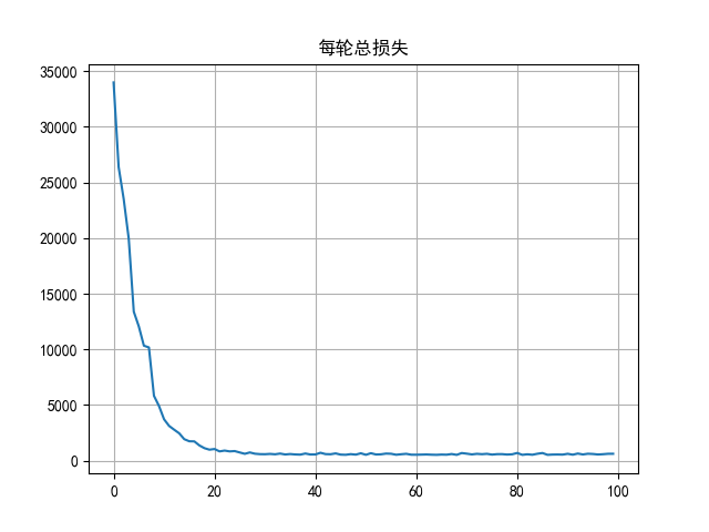
前向传播:数据从输入层进入,经过每一层的权重计算和激活函数,最后得到一个预测值。我们将预测值与真实值对比,计算出损失(Loss/Error)。
反向传播:从损失函数出发,逆向计算损失对每一层参数(权重 w 和偏置 b)的梯度。
基本使用
sum():计算张量中所有元素的总和
backward():反向传播计算梯度
1 | |
注意:
要从设置了requires_grad = True的tensor中获取ndarray,需要使用x.detach().numpy()来获取
1 | |
代码
线性回归案例
1 | |
激活函数
作用是为神经网络引入非线性因素,如果没有激活函数,输出都是输入的线性组合,与没有隐藏层效果相当
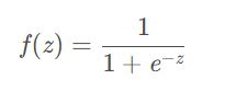
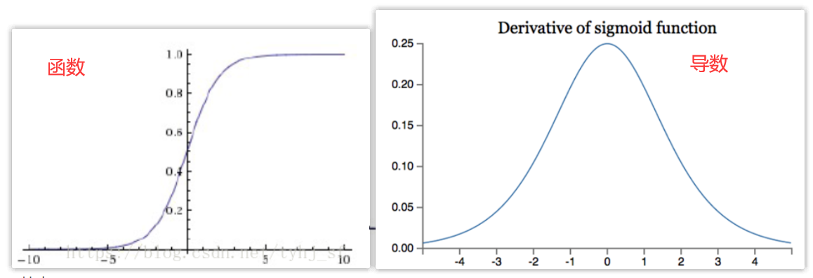
Sigmoid
作用:把输入值映射到[0, 1]区间上,多用于二分类
缺点:
- Sigmoid的导数最大值为0.25,反向传播时会让值变小,在多层的神经网络中会导致梯度消失
- 只能用于浅层网络
- 幂运算相对耗时
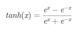
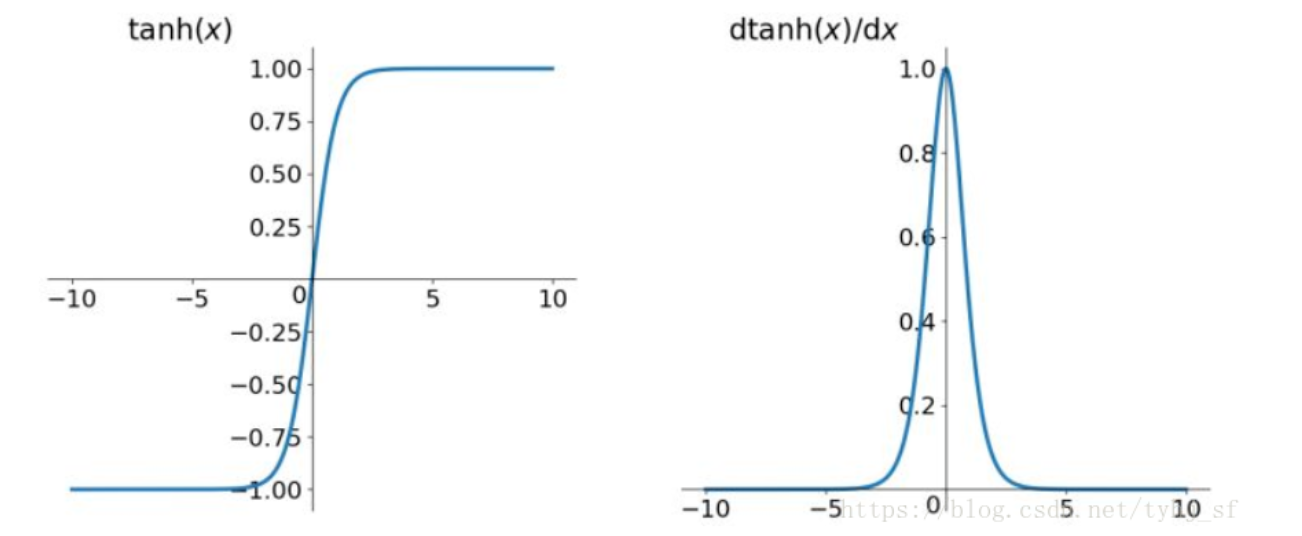
Tanh
作用:把输入值映射到[-1, 1]区间上
优点:
- 梯度大,比Sigmoid收敛速度快
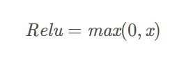
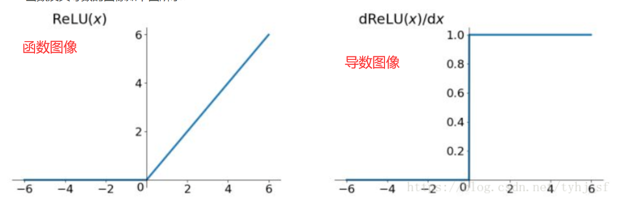
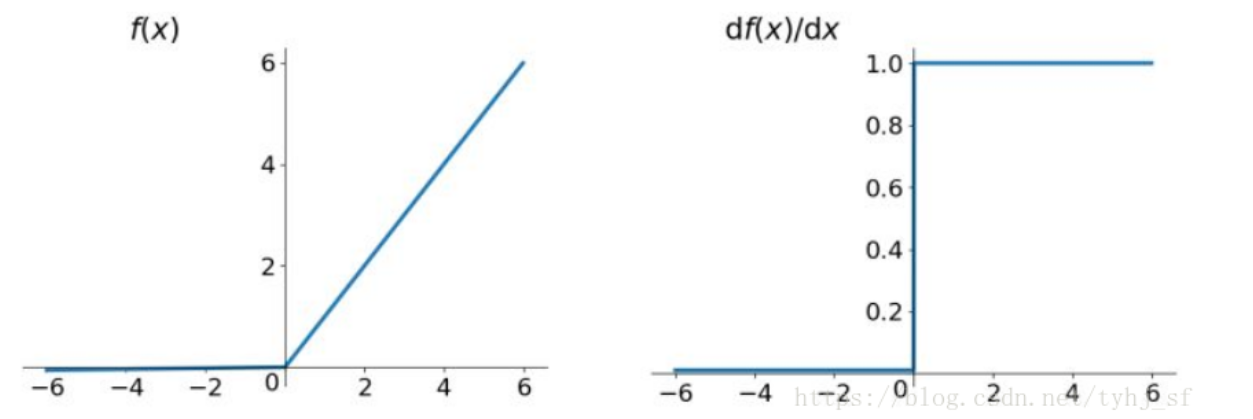
ReLU
作用:只取正数
优点:
- 简单效果好,计算速度快
- 收敛速度快于Sigmoid和Tanh
缺点:
- Dead ReLU Problem:指的是某些神经元可能永远不会被激活,导致相应的参数永远不能被更新
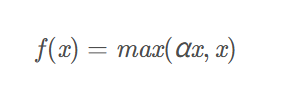
Leaky ReLU
作用:将ReLU的前半段设为αx而非0,通常α = 0.01,解决ReLU的Dead ReLU Problem
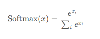
Softmax
作用:用于多分类,是Sigmoid的推广;选择概率最大的为输出
神经网络搭建
参数初始化
给每个神经元的权重和偏置赋予一个初始值的过程
常用的初始化方式:
- 全0/1初始化
- 将所有的权重设为0/1
- 问题:会导致对称性问题。反向传播时每一层的梯度都相同,网络退化为一个单神经元模型。
- 随机初始化
- 从正态分布或均匀分布中随机采样
- 使用场景:浅层网络或简单的实验
- Xavier 初始化
- 为了保持信号在穿过每一层网络时方差不变,,从而避免梯度消失或爆炸,适用于 Sigmoid / Tanh
- He 初始化
- 为了保持信号在穿过每一层网络时方差不变,,从而避免梯度消失或爆炸,适用于 ReLU
损失函数
多分类交叉熵损失函数
Cross-Entropy Loss,用于多分类任务
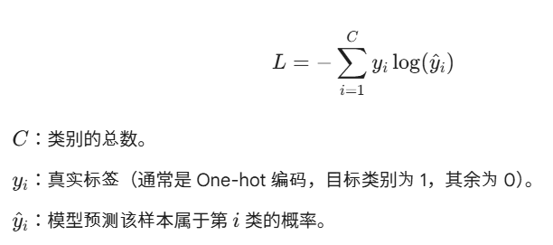
- 预测值是将最后的输出值通过Softmax激活函数得来
- 因此最后输出层不用激活函数
- 经过
log()后,如果模型给正确类别预测的概率接近1,那么损失函数接近0 - 如果模型给正确类别预测的概率越小,那么损失函数接近无穷大
二分类任务损失函数
Binary Cross-Entropy Loss,简称 BCE
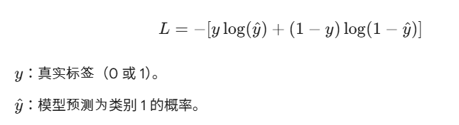
- 模型预测为类别为1的概率
- 标签为1时看左边,预测值越大,损失越小
- 标签为0时看右边,预测值越小,损失越小
回归任务损失函数
Mean Absolute Error(MAE),平均绝对误差,也称为L1 Loss
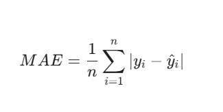
- 优点:对离群点更具鲁棒性,不会像 MSE 那样被极值带偏。
- 缺点:在误差接近0的地方导数不连续(不可导),这可能导致模型在收敛最后阶段出现震荡。
Mean Squared Error(MSE),均方误差,也称为L2 Loss,最常用
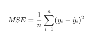
- 通过平方放大误差。如果预测值离真实值很远,损失会迅速增加。
- 优点:数学性质极佳(处处可导),有利于使用梯度下降法求解。
- 缺点:对离群点非常敏感。如果数据中有一个极端的噪声点,MSE 会为了弥补这个大误差而带偏整个模型。
Huber Loss,平滑平均绝对误差
- 是 MSE 和 MAE 的折中方案,结合了两者的优点
- 当误差较小时,它像 MSE,解决L1零点不可导的问题
- 当误差较大时,它像 MAE,解决L2离群点导致的梯度爆炸问题
代码
参数初始化示例
1 | |
神经网络搭建示例
1 | |
多分类交叉熵损失函数示例
1 | |
二分类任务损失函数示例
1 | |
回归任务损失函数
1 | |
神经网络优化
概念
- Epoch:1个Epoch = 使用全部数据进行1轮训练
- Batch_size:使用部分样本进行训练的样本数大小
- 反向传播步骤:
- 计算误差:在前向传播结束时,通过损失函数算出预测值和真实值的差距。
- 梯度追踪:利用微积分中的链式求导法则,从后往前计算损失函数对每一个参数(权重W和偏置b)的导数(即梯度)。
- 更新参数:优化器根据这些梯度,把参数往“误差变小”的方向推一小步
- 指数加权平均:计算平均数时,每个数的权重不同,越远的数权重越小
梯度下降的优化
Momentum
在普通的 SGD 中,参数更新只取决于当前的梯度,可能会导致:
- 梯度来回震荡
- 在鞍点(导数为0的点)停住不更新
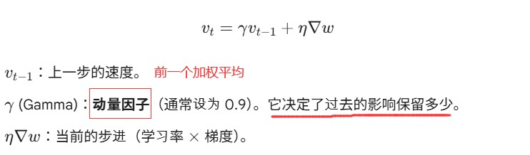
- 当前权重的更新不再只参考当前梯度,而是也参考之前的梯度
- 越近的梯度权重越大
- γ值越大,过去的梯度的影响越大,为0则等价于小批量梯度下降
- 通过添加了一个正则项,解决了鞍点不更新的问题
AdaGrad
对频繁出现的特征进行用小学习率更新,偶尔出现的特征用大学习率更新
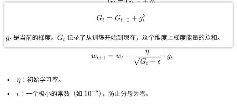
步骤:
- 对每个权重,累计梯度的平方
- 在更新权重的时候,作为学习率的分母
- 这样频繁更新的权重学习率就小,偶尔更新的权重学习率就大
- 随着训练的进行,学习率会越来越小,做到前期大步探索,后期细微调整
缺点:后期学习率过小,更新缓慢
RMSProp
只记录最近一段时间的累计梯度,解决AdaGrad在后期学习率过小的问题
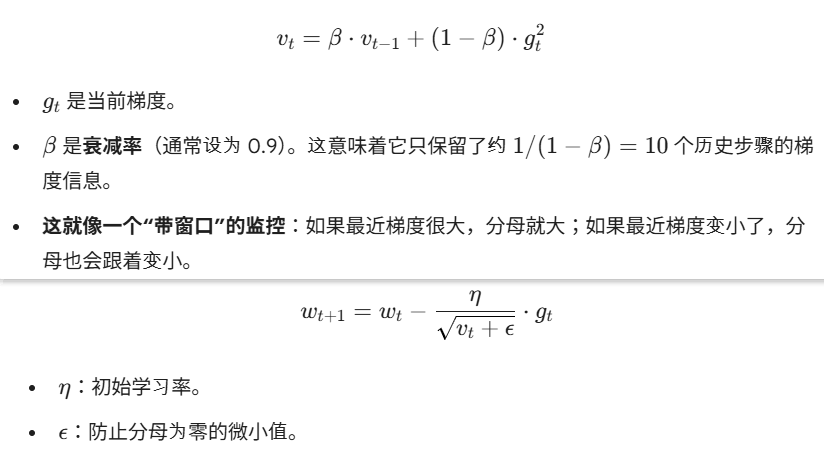
步骤:
- 计算梯度平方的指数移动平均
- 使用指数移动平均来降低以前梯度的权重
✨Adam
Momentum优化梯度、RMSProp更新学习率
Adam是Momentum和RMSProp的结合
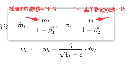
- 上面的公式是为了在开始训练时,解决指数移动平均还是0导致的更新慢问题
- 刚开始训练轮次t很小,分母也小,就放大了整个值
- 随着训练轮次t的增加,分母会逐渐趋于1,就不会继续放大
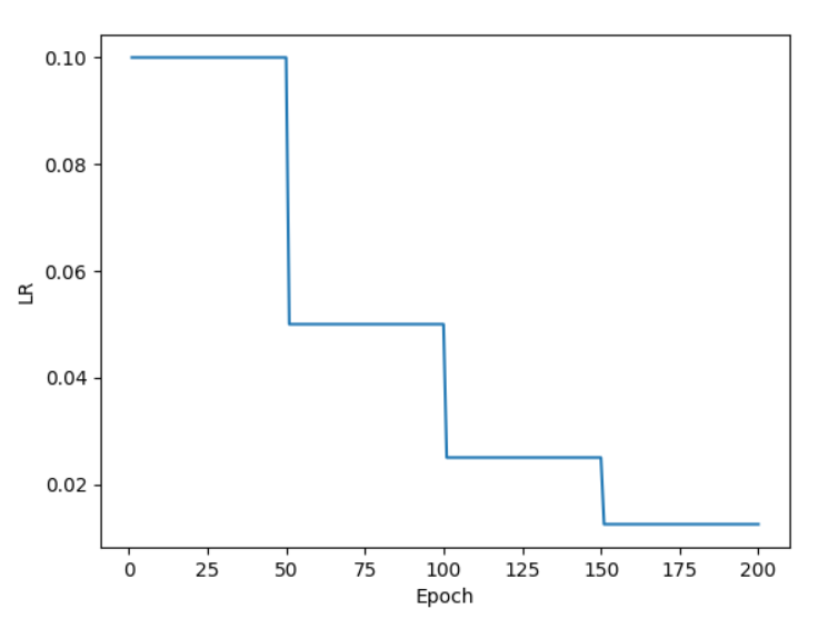
学习率衰减
在训练初期,模型离最优解很远,大的学习率可以更快向最优解收敛;
在训练后期,为了防止在两点间震荡,应当使用小的学习率
- 等间隔衰减:每隔固定的epoch就衰减一次
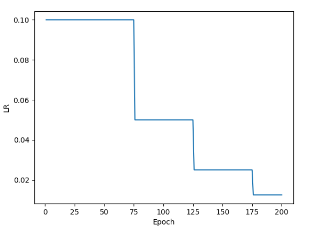
- 指定间隔衰减:在指定的训练轮次后衰减一次
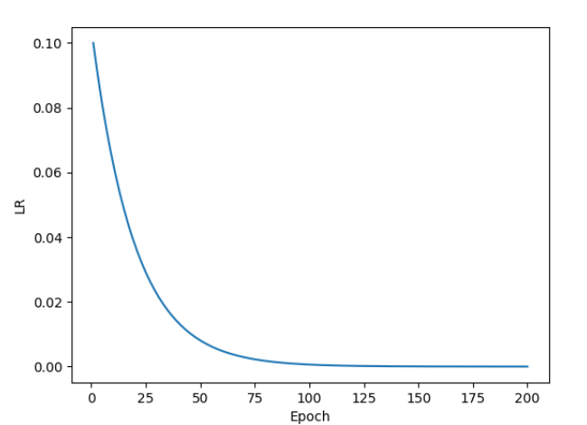
- 按指数学习率衰减:让学习率随着训练轮数呈指数级减少
正则化
防止模型过拟合
Dropout正则化
Batch Normalization, BN,在神经网络的训练过程中,以一定的概率p(通常0.2~0.5),随机将一部分神经元的输出置为 0
通常放在激活函数后
训练阶段:按照概率p随机丢弃神经元,被丢弃的神经元在本批次中不会被更新
测试阶段:不丢弃任何神经元,因为训练时只用了一半神经元,测试时全用会导致输出数值偏大。因此,在训练时通常会输出 / (1 - p)来放大输出,从而保证测试时不需要做额外处理。
批量归一化
作用是确保每一层神经网络的输入始终保持稳定的分布
通常放在激活函数前
步骤:
计算这层神经元的输出的期望和方差
将输出处理成均值为0、方差为1的标准分布
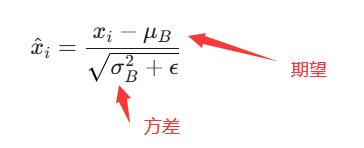
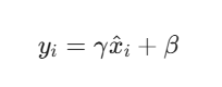
平移和缩放
代码
动量法Momentum示例
1 | |
AdaGrad示例
1 | |
RMSProp示例
1 | |
Adam示例
1 | |
等间隔衰减示例
1 | |
指定间隔衰减示例
1 | |
按指数学习率衰减示例
1 | |
Dropout示例
1 | |
批量归一化示例
1 | |
CNN
Convolutional Neural Network,卷积神经网络
实例代码
预测手机价格区间(多分类任务)
1 | |