机器学习
机器学习
概述
人工智能三大概念
- 人工智能:AI,Artificial Intelligence
- 机器学习:ML,Machine Learning
- 深度学习:DL, Deep Learning
包含关系:人工智能 > 机器学习 > 深度学习
AI发展三要素
数据、算法、算力
样本、特征、标签
- 样本(Sample):一行数据就是一个样本;多个样本组成数据集;有时一条样本被叫成一条记录
- 特征(feature) :一列数据一个特征,有时也被称为属性
- 标签/目标(label/target) :模型要预测的那一列数据
- 训练集(training set):训练模型的数据集
- 测试集(testing set):测试模型的数据集,和训练集的比例一般为8:2或7:3
监督学习
有监督学习:输入的训练数据有标签的
- 分类问题:标签值是不连续的
- 回归问题:标签值是连续的
无监督学习:输入数据没有被标记,即样本数据类别未知,没有标签;
根据样本间的相似性对样本集进行聚类
机器学习流程
获取数据
数据基本处理
缺失值处理、异常值处理等
特征工程
特征提取、预处理、降维等
模型训练
线性回归、逻辑回归、决策树、GBDT等
模型评估
特征工程
- 特征提取
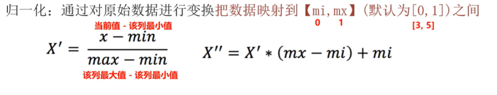
- 特征预处理:解决因量纲问题,导致有些特征对模型影响大、有些影响小
- 归一化:(当前值 - 最小值)/(最大值 - 最小值)
- 标准化
- 特征降维
- 特征选择
- 特征组合
机器学习库
- 官网:https://scikit-learn.org/stable/
- 安装:
pip install scikit-learn
KNN算法
K Nearest Neighbor,K邻近算法
思想
- 计算和样本的距离,找出最近的K个,按距离排序;
- 如果是分类问题,则这K个里哪种分类最多就为哪个(一样多选最近的)
- 如果是回归(预测)问题,则取这K个的均值
计算距离可以有多种方式,如欧式距离、曼哈顿距离等
K值选择
- 过小会导致过拟合
- 过大会导致欠拟合
代码实现
分类代码实现
1 | |
回归代码实现
1 | |
距离度量方式
- 欧式距离:类似勾股定理,对应特征的差值平方,求和再开根号
- 曼哈顿距离:abs(对应维度差值)之和
- 切比雪夫距离:max(对应维度差值的的绝对值)
特征预处理
解决量纲问题导致放差值相差较大,影响模型的最终结果
归一化:将值映射到指定区间里,容易受极值影响,适合小数据集
1
2
3
4
5
6
7
8
9
10
11
12
13
14from sklearn.preprocessing import MinMaxScaler
x_train = [[90, 2, 10, 40], [60, 4, 14, 45], [75, 3, 13, 46]]
# 归一化对象, 默认[0, 1]
scaler = MinMaxScaler(feature_range=(0, 1))
# 进行归一化操作
x_train_new = scaler.fit_transform(x_train)
print(x_train_new)
# [[1. 0. 0. 0. ]
# [0. 1. 1. 0.83333333]
# [0.5 0.5 0.75 1. ]]标准化:将数据转化为标准正态分布,可以减少极值的影响,适合大数据集
(当前值 - 均值) / 标准差
1
2
3
4
5
6
7
8
9
10
11
12
13
14from sklearn.preprocessing import StandardScaler
x_train = [[90, 2, 10, 40], [60, 4, 14, 45], [75, 3, 13, 46]]
# 标准化对象
scaler = StandardScaler()
# 进行标准化化操作
x_train_new = scaler.fit_transform(x_train)
print(x_train_new)
# [[ 1.22474487 -1.22474487 -1.37281295 -1.3970014 ]
# [-1.22474487 1.22474487 0.98058068 0.50800051]
# [ 0. 0. 0.39223227 0.88900089]]
实例
鸢尾花分类
1 | |
超参数选择方法
网格搜索
交叉验证:
- 将训练集平均划分为N份(通常称N为折数),N - 1份作为训练集,1份作为验证集
- 每次拿不同的1份作为测试集,总共训练N次
- 将N轮得到的性能指标取平均值,这个平均值就是最终评估分数
网格搜索:
将若干超参数可能得取值传递给网格搜索对象,会自动完成不同超参数的组合
如超参数A可取值[0, 1, 2], 超参数B可取值[3, 4]
则超参数的组合有3 * 2 = 6种
对每组超参数都采用交叉验证,最后选出最优的
案例
1
2
3
4
5
6
7
8
9
10
11
12
13
14
15
16
17
18
19
20
21
22
23
24
25
26
27
28
29
30
31from sklearn.datasets import load_iris #加载鸢尾花测试集的.
from sklearn.model_selection import train_test_split, GridSearchCV #分割功练集和测试集的
from sklearn.preprocessing import StandardScaler #数据标准化的
from sklearn.neighbors import KNeighborsClassifier #KNN算法分类对象
from sklearn.metrics import accuracy_score # 模型评估
# 加载数据集
iris = load_iris()
# 分割训练集和测试集
x_train, x_test, y_train, y_test = train_test_split(iris.data, iris.target, test_size=0.2, random_state=42)
# 数据预处理
scaler = StandardScaler()
x_train = scaler.fit_transform(x_train)
x_test = scaler.transform(x_test)
# 模型
estimator = KNeighborsClassifier()
# 超参数可能的取值
param_dict = {'n_neighbors': [i for i in range(1, 11)]}
# cv: 交叉验证的折数, 返回处理后的模型
estimator = GridSearchCV(estimator=estimator, param_grid=param_dict, cv=4)
# 训练模型
estimator.fit(x_train, y_train)
print(f'最优评分: {estimator.best_score_}')
print(f'最优超参组合: {estimator.best_params_}')
print(f'最优的估计器对象: {estimator.best_estimator_}')
print(f'具体的交叉验证结果: {estimator.cv_results_}')
手写数字识别
绘制数字
1 | |
训练和保存模型
1 | |
使用保存的模型
1 | |
线性回归
用线性公式来描述多个自变量(特征)和一个因变量(标签)之间的关系
属于有监督学习,标签是连续的
概念
- 一元线性回归:y = wx + b(w为权重,b为偏置),目标值与单个因变量有关
- 多元线性回归:y = (w1x1 + b1) + (w2x2 + b2) + … + b,目标值与多个因变量有关
目标是找出能使损失函数最小的权重和偏置
损失函数
Loss Function, 用来评判模型的好坏,值越小表示误差越小
损失函数种类
- 均方误差(MSE):(预测值 - 真实值)^2求和 / 样本总数
- 平均绝对误差(MAE):|预测值 - 真实值|求和 / 样本总数
- 均方根误差(RMSE):均方误差的值开根号
找让损失函数最小的权重和偏置的方法
最小二乘法
最小二乘法可以直接计算出最优的w和b,前提是数据量不大,且方程有解析解
一元线性回归的情况:
- 损失函数分别对w(权重)和b(偏置)分别求偏导
- 然后联立起来求偏导为0的值,来让损失函数最小
多元线性回归的情况:
- 多元线性回归方程式:y = w1x1 + w2x2 + w3x3 + … + b = w^Tx + b
- 把一个样本的特征值带入x1、x2、….得预测值
- 损失函数 = 累加每个样本的(真实值 - 预测值)^ 2
对损失函数的w(包含所有权重的矩阵)求导,得到方程
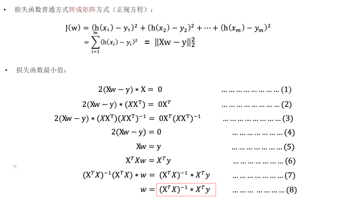
可知要求w时X^(-1)要存在,不是所有情况都能用
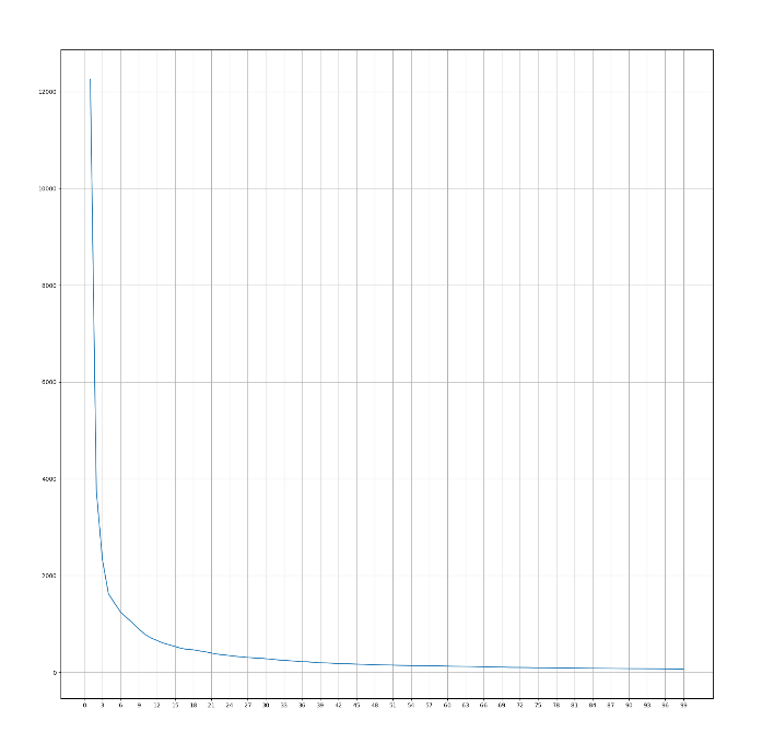
✨梯度下降法
沿着梯度下降的方向求解极小值
一元线性回归的情况:
- 随机初始化 w 和 b,确定一个学习率α,选择迭代次数
- 在每一步迭代中,使用当前 w 和 b 计算损失函数对 w 和 b 的偏导数(梯度)
- 沿梯度的反方向更新w和b(梯度的方向是上升最快的方向)
- 直到迭代了设置的迭代次数、或者损失函数收敛到了指定的阈值内时停止
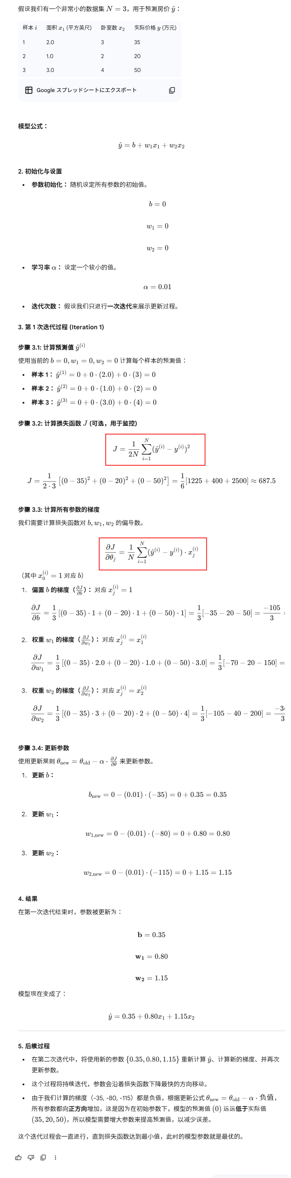
多元线性回归的情况:
对所有的参数求偏导,然后同时更新
梯度下降法例子
梯度下降法分类
根据每轮迭代中用于计算梯度的样本数量来分类
批量梯度下降法(Batch(Full) Gradient Descent, BGD/FGD)
定义:使用全部训练数据来计算损失函数的梯度
优点:能保证收敛到全局最优解
缺点:速度慢,内存占用大
随机梯度下降法 (Stochastic Gradient Descent, SGD)
定义: 每次参数更新时,只使用随机的一个训练样本来计算梯度
优点:计算速度快
缺点:收敛性较差,通常只能震荡地接近最优解
✨小批量梯度下降法 (Mini-Batch Gradient Descent, MBGD)
定义:每次参数更新时,使用一小批(Mini-Batch)训练样本(通常是 32、64、128 等)来计算梯度
优点:结合和BGD和SGD的特点
欠拟合和过拟合的解决方法
欠拟合的成因:学习到数据的特征过少
欠拟合的解决方法:添加特征、添加多项式特征项
过拟合的成因:特征过多,存在一些嘈杂特征
过拟合的解决方法:重新清洗数据、增大数据量、正则化、减少特征数量
正则化
过拟合时,模型往往会给某些特征极大的权重、专门去迎合训练数据中的噪声
正则化的作用是让权重的值不要太大
L1正则化
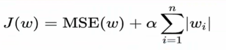
- α为惩罚系数,即权重大的时候对损失函数的影响
- 可能会让一些权重值直接变成0(在特征很多需要降维时使用)
L2正则化
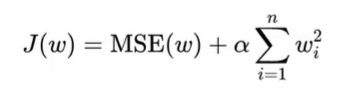
- 对权重的调整更平滑一些,一般不会变为0
代码
正规方程
1 | |
梯度下降法
1 | |
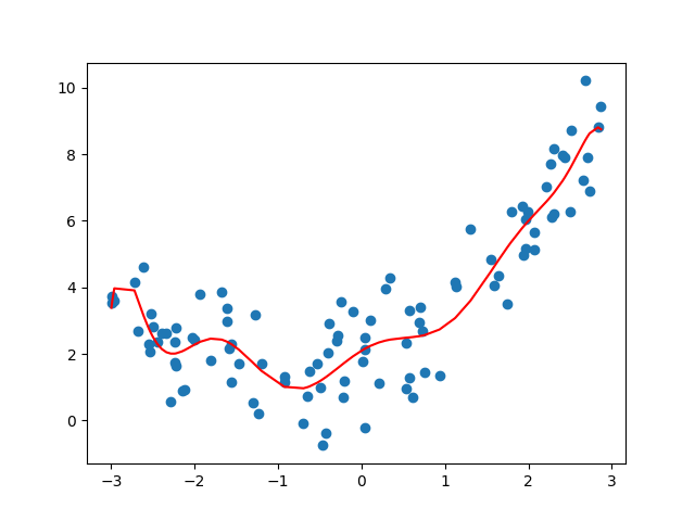
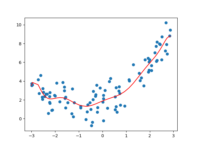
欠拟合
1 | |
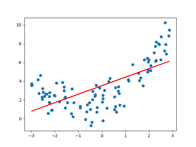
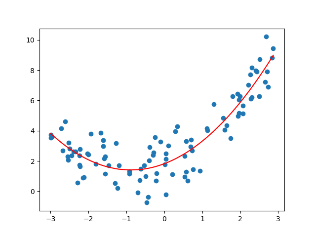
拟合
1 | |
过拟合
1 | |
正则化
1 | |

逻辑回归
有监督学习,标签是离散的
概念
逻辑回归的作用:分类
Sigmoid激活函数:
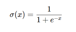
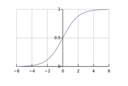
作用:把数映射到[0, 1]区间上,来表示样本属于某一类的概率
最大似然估计:找一组参数,让已经发生的这些数据在这个模型下看起来最合理、最有可能发生
损失函数
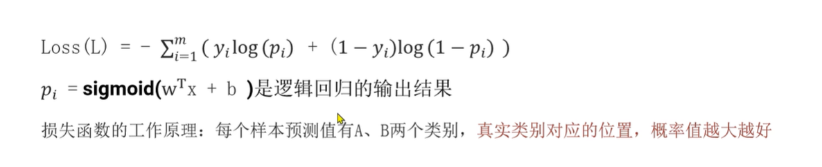
- 如果y标签为1,则只会计算函数左边那块
- 如果y标签为0,则只会计算函数右边那块
- 注意到前面有个符号,则概率值越大,损失函数越小
分类的评估方法
使用准确率来评估太粗糙了,正类和负类同等重要,错一次的代价是一样的;
准确率看不出来预测错的类型是什么,
例如预测是否生病,1000个人中只有一个人真生病,模型只会输出没生病,准确率就高达99.9%
混淆矩阵
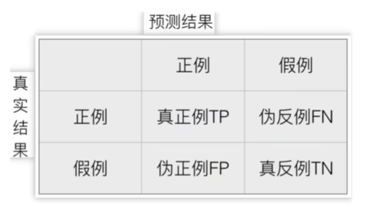
- 精确率:TP / (TP + FP),预测结果为正中,对的占比
- 召回率:TP / (TP +FN),正例中被预测为正的占比
- F1-score:2 * 精确率 * 召回率 / (精确率 + 召回率)
代码
逻辑回归实例1
1 | |
混淆矩阵
1 | |
逻辑回归实例2
one hot编码:为每个类别创建一个独立的二进制特征列,用 1 表示样本属于该类别,用 0 表示不属于。比如把颜色拆分为是否为红色,是否为绿色,是否为蓝色;
作用:适配机器学习算法, 若直接类别1=1、类别2=2、类别3=3,模型可能会误认为类别3 > 类别2 > 类别1
1 | |
决策树
概念
什么是决策树:树中每个非叶子节点表示一个特征上的判断,每个分支表示一个判断结果的输出,每个叶子节点代表一种分类结果
建立决策树过程:
- 特征选择:选取有较强分类能力的特征
- 生成决策树
- 剪枝:解决过拟合问题
种类
ID3决策树
偏向于选择种类多的特征
概念
信息熵计算方法:-Σ(标签分类占比)*log(标签分类占比)
信息熵越大代表越混乱
条件熵计算方法:在已知特征 X 的条件下,目标变量 Y 的不确定性
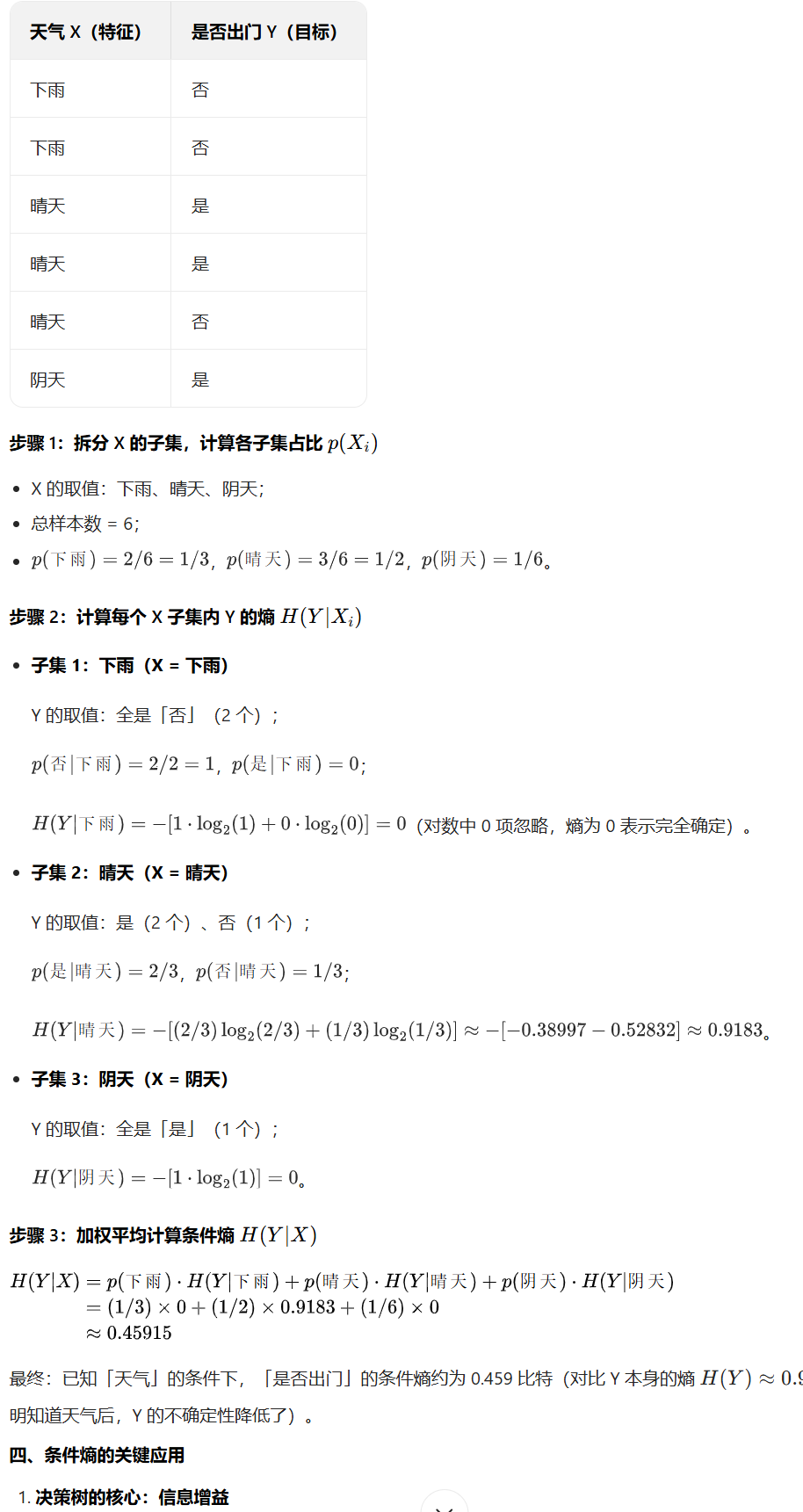
信息增益 = 信息熵 - 条件熵
建树过程
- 计算每个特征的信息增益
- 使用信息增益最大的特征,将该数据集拆分为多个子集
- 使用该特征值作为决策树的一个节点
- 对每个子集,使用剩余的特征重复上述过程
- 当这个分支的所有数据都只有一个标签时,这个分支终止,叶子结点为这个标签
C4.5决策树
解决ID3决策树过拟合的问题
ID3决策树偏向于选择种类多的特征,而信息增益率偏向于选择种类少的特征
概念
- 特征熵:算特征列的熵
- 信息增益率=信息增益 / 特征熵
建树过程
和ID3树类似,只是将信息增益换成信息增益率
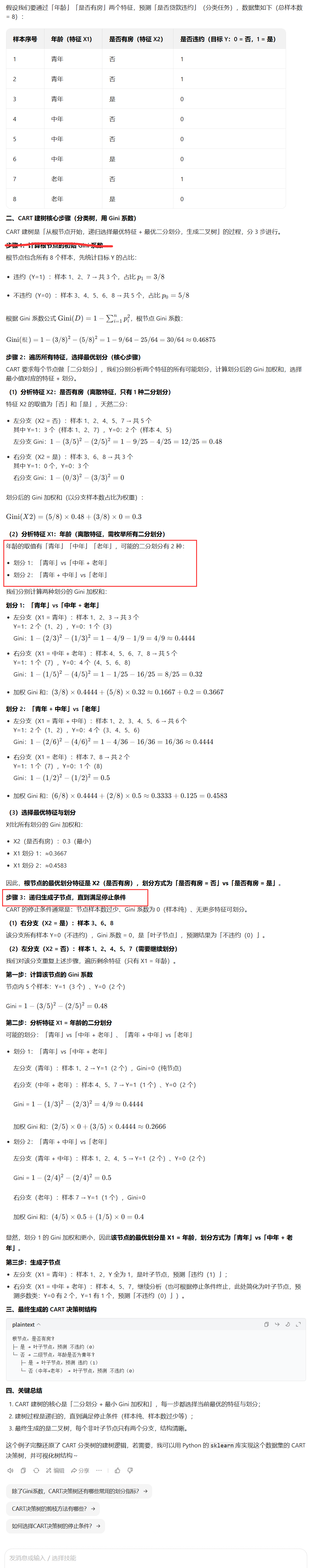
CART决策树
Classification and Regression Tree,分类与回归树,最常用的决策树算法之一,核心特点是既能做分类任务,也能做回归任务
概念
基尼值:从数据集中随机抽取两个样本,类别标记不一致的概率
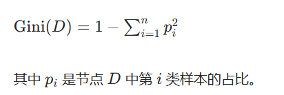
- 基尼值越小,节点的纯度越高
基尼指数:一个特征中,Σ(某个取值对应的基尼值 * 这种取值的占比)
✨分类树建树过程
CARF要求每个节点做二分划分,分别分析所有特征的所有可能划分
如果特征值是连续的,将数值做升序排序,以相邻值的中点作为二分位置
计算划分后的Gini指数
选择最小值对应的特征的划分
下一次节点分裂时,和前面的决策树不同,用过的特征仍然可以再用
回归树建树过程
- 分裂依据是最小化节点分裂后的总平方误差(MSE)
- 节点的MSE就是每个样本的真实值和节点均值的误差平方和
- 分裂点的选择为,将某个特征的特征值按升序排序,每两个值的中间值选为分裂点
- 遍历所有特征和该特征可能的阈值,选择MSE最小的组合来进行分裂
预测
将样本沿着树的分叉走,直到到达叶子结点。
如果是分类问题:叶子节点所有样本的标签中,最多的即作为预测值
如果是回归问题:叶子节点所有样本的标签的均值即作为预测值
剪枝
- 预剪枝:在划分前进行估计,如果不能带来决策树泛化能力提升,则停止划分
- 优点:降低了过拟合的风险,减少了决策树的训练时间
- 缺点:带来了欠拟合的风险
- 后剪枝:训练完后,自底向上对非叶子节点进行考察,若将该节点替换为叶子结点能提升泛化能力,则替换
- 优点:泛化能力优于预剪枝
- 缺点:训练开销大得多
代码
分类决策树案例
数据集下载:https://tianchi.aliyun.com/dataset/179968
1 | |
回归决策树案例
回归用的较多的还是线性回归
1 | |
集成学习
通过多个模型的组合形成一个精度更高的模型
训练时,使用训练集依次训练出弱学习器,对未知的样本进行预测
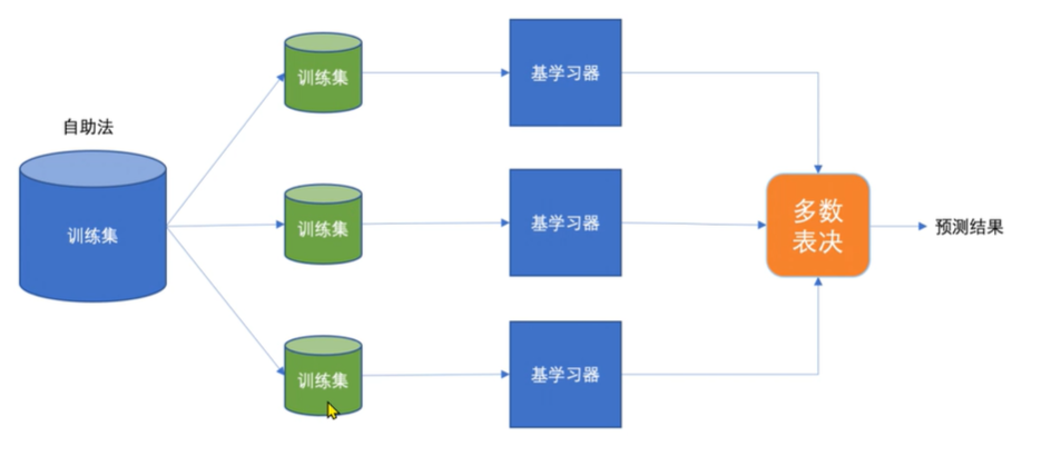
并行式集成(Bagging)
训练过程:
- 从原始数据集中,通过自助采样(有放回地随机选样本)生成多个不同的子数据集。
- 用每个子数据集训练一个独立的基模型(比如决策树)。
- 最终预测时,分类问题取多数投票,回归问题取平均值。
随机森林算法
- 每次有放回的抽取若干个样本
- 选取部分特征来学习,默认是CART树
- 构建多颗这样的树
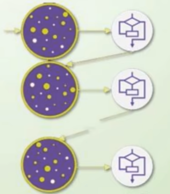
串行式集成(Bossting)
训练过程:
- 先训练一个基模型,对样本进行预测。
- 提高预测错误的样本的权重,让下一个基模型重点学习这些难样本。
- 重复上述过程,生成多个基模型,最终按权重融合
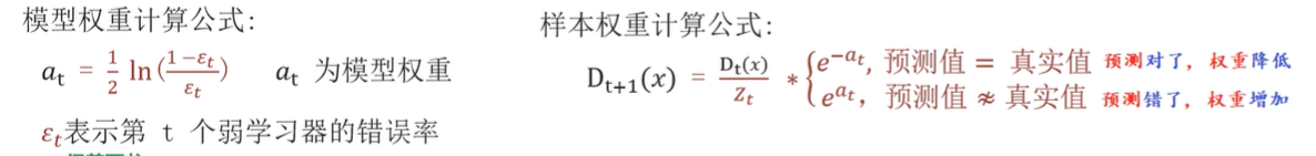
Adaboost算法
开始时所有样本权重相同,模型会优先拟合权重高的样本
权重在算当前错误率的时候用,若某个样本预测错了,错误率就会加上这个权重
因此会尽量先拟合权重高的样本
共训练T轮,每轮都用到全部训练集,T为学习器(仅包含一个分裂节点的决策树)的数量,每个学习器也有权重
每轮训练后,预测错误的样本权重会升高,对的会降低,权重会传给下一个学习器
最后将这些学习器合成一个强模型,通过加权投票来给出结果
GDBT算法
Gradient Boosting Decision Tree,梯度提升决策树
逐步拟合前一轮模型的残差
以回归为例
初始化弱学习器:取(训练时的)标签的均值为预测值,使初始损失最小
- 找到使得负梯度(目标值 - 预测值)均方误差最小的切分点,将样本分到两个叶子结点中
- 预测时根据特征值判断到哪个叶子接点中,预测值为样本标签的均值
将上一轮的负梯度(残差)作为下一轮的标签,继续重复上面的操作
训练完后,预测时是把测试集给每个弱学习器,累加每个的输出值即为预测值
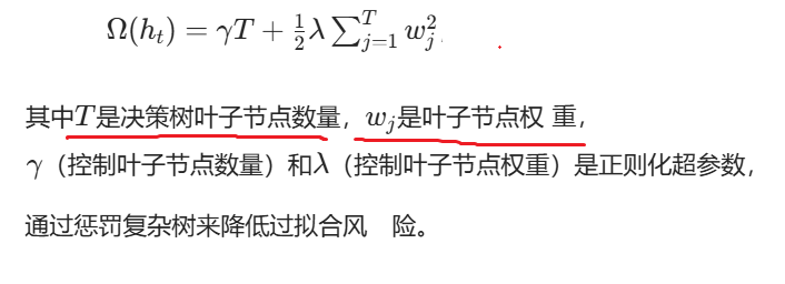
XGBoost算法
eXtreme Gradient Boosting,极端梯度提升
在 GBDT 的基础上,增加了正则化项,用于约束模型复杂度,避免过拟合
初始化模型
迭代训练弱决策树
计算当前模型的一阶导数和二阶导数,作为拟合目标;
基于特征并行优化,为当前决策树寻找最优分裂点);
生成新的弱决策树,并通过正则化项约束树的复杂度;
只有分裂后损失值下降的足够多才允许分裂;还会尽量选择多个小权重叶节点,而非少数大权重叶节点
确定该树的权重,将其加入强模型,更新整体预测结果。
有弱树加权累加后,得到最终强模型
代码
随机森林实例
1 | |
Adaboost算法实例
1 | |
GBDT算法实例
1 | |
XGBoost算法实例
需要安装pip install xgboost
1 | |
朴素贝叶斯算法
朴素贝叶斯是有监督的分类算法,它的本质是:利用贝叶斯公式,结合「特征独立」的朴素假设,计算样本属于每个类别的后验概率,最终选择概率最大的那个类别作为预测结果。
原理
朴素贝叶斯基于条件概率公式:
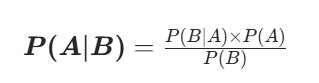
朴素的含义是:特征之间是互相独立的
预测步骤:
- 通过分词器提取样本中关键字作为特征
- 根据概率公式,计算在有这些特征的条件下,是某个标签的概率
- 取概率最大的标签作为预测值
代码
贝叶斯算法实例
安装分词器:pip install jieba
1 | |
聚类算法
无监督学习,根据样本的内在相似性,把数据划分成若干个簇(Cluster)
概念
相似性的度量方法:
- 距离度量:欧式距离(最常用)、曼哈顿距离、余弦相似度
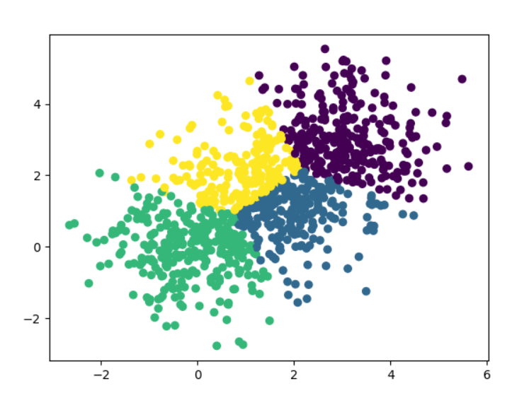
KMeans
是划分式聚类中最经典、最常用的无监督学习算法,核心目标是:给定 k 个簇的数量,将数据集划分为 k 个簇,使得簇内样本的相似度最高,簇间样本的相似度最低
步骤:
- 随机选择k个样本点作为聚类中心
- 每个样本选择最近的中心聚集成簇
- 每个簇算出自己的中心点(不一定是样本点)
- 之后用这个新的中心的重新聚类
- 重复上面过程,直到生成的中心点和上次一样时停止
评估指标
误差平方和SSE
SSE = 簇内每个点到质心距离的平方和,所有簇之和
值越小越好
轮廓系数法SC
计算一个样本到簇内其他样本的平均距离a
计算一个样本到最近簇内其他样本的平均距离b
轮廓系数 = (b - a) / max(a, b),范围为[-1, 1]
计算所有样本的平均轮廓系数,值越大聚类效果越好
代码
KMeans实例
1 | |
SSE值
1 | |