python基础

基本语法

注释

单行：#

多行：'''或"""

# 如果一段代码太长，可用\分段
a = b + c + \
	d + e + \
    f

变量类型

查看类型

type()查看变量类型

isinstance(a, (类型1, ...))判断是否是其中一种类型或子类

数字

• int
• bool（True/False）
• float
• complex（复数）

/返回浮点数，//返回整数的部分

字符串

单行字符串可用''或""，多行字符串可用''' '''或""" """

转义符号\

不让\生效，在引号前加r

可用+连接字符串，*重复字符串

字符串是不可改变量

切片

左闭右开

-1为末尾位置

还可加上步长，步长-1表示逆向

格式化

print ("我叫 %s 今年 %d 岁!" % ('小明', 10))

# 还有前面加f的格式化语法
name = 'aaa'
print(f'Hello {name}')      # Hello aaa

w = {'name': 'baidu', 'url': 'www.baidu.com'}
print(f'{w["name"]}: {w["url"]}')   # baidu: www.baidu.com

列表

列表的元素是可改变的

a = [1, 2, 3, 4, 5, 6]
print(a[1 : 2]) # [2]
print(a[1 :])   # [2, 3, 4, 5, 6]

a[1] = 0
print(a) #[1, 0, 3, 4, 5, 6]

列表操作

# 增加元素
list1 = [1, 2, 3]
list1.append(4)
print(list1)    # [1, 2, 3, 4]

# 删除元素
del list1[0]
print(list1)    # [2, 3, 4]

# 比较列表
import operator

list1 = [1, 2, 3, 4, 5, 6, 7, 8, 9, 10]
list2 = [1, 2, 3, 4, 5, 6, 7, 8, 9]
print(operator.eq(list1, list2))	# False

元组

元组的元素不可以改变

可以把字符串看成特殊的元组

tup = (1, ) # 只包含一个元素的元组
a = (1)     # int类型
b = () 		# 空元组
print(type(tup))    # <class 'tuple'>
print(type(a))  	# <class 'int'>

集合

集合的元素可变，唯一

创建可用{}或set()，空集合要用set

a = set('abracadabra')
b = set('alacazam')

print(a)

print(a - b)     # a 和 b 的差集

print(a | b)     # a 和 b 的并集

print(a & b)     # a 和 b 的交集

print(a ^ b)     # a 和 b 中不同时存在的元素

字典

创建可用{}或dict，空字典可用{}创建

key必须为不可变类型（数字、字符串、元组、布尔等）

a = {'a': 1, 'b': 2, 'c': 3, 4 : 'd'}
print(a)        # {'a': 1, 'b': 2, 'c': 3, 4: 'd'}
print(a['a'])   # 1
print(a[4])     # d

字典操作

# 删除指定key
d = {1 : 1, 2 : 2, 3 : 3}
del d[1]
print(d)    # {2: 2, 3: 3}

# 清空字典
d.clear()
print(d)    # {}

输入输出

# 输入
price = input("Enter price: ")

# print默认带换行
print(price)
print(price, end = '')

format格式化

# 按位置填充
print("Hello, {}!".format("Alice"))
print("Hello, {0}, you are {1} years old.".format("Bob", 25))

# 按关键字填充
print("Site name: {name}, Rank: {rank}".format(name="Google", rank=1))

# 混合字典访问
user = {"name": "Alice", "age": 18}
print("Name: {0[name]}, Age: {0[age]}".format(user))

# 解包
data = {"site": "Google", "rank": 1}
print("Site: {site}, Rank: {rank}".format(**data))

格式化控制符

格式符	含义	示例值	示例结果
d	十进制整数	{0:d}	42
f	浮点数（默认 6 位）	{0:f}	3.141593
.2f	保留 2 位小数	{0:.2f}	3.14
>10	右对齐，占 10 宽度	{0:>10}	text
<10	左对齐，占 10 宽度	{0:<10}	text
^10	居中，占 10 宽度	{0:^10}	text
,	千位分隔符	{0:,}	1,000,000
%	百分比（乘以 100）	{0:.2%}	25.00%

条件/循环

• if / elif / else

• match…case(相当于switch…case，在3.10版本可用)

  status = 400
  match status:
      case 400 | 401 | 402:
          return "Bad request"
      case 404:
          return "Not found"
      case 418:
          return "I'm a teapot"
      case _:
          return "Something's wrong with the internet"

• while…else

• for…in…else

  range(5): 遍历从0到4

• pass: 空语句，不做任何事

导入模块

导入模块的搜索路径：

1. 当前目录
2. 环境变量 PYTHONPATH 指定的目录
3. Python 标准库目录
4. .pth 文件中指定的目录

# 整个模块
import sys

# 模块中的某个函数
from sys import argv, path

# 模块中的所有函数(不推荐，容易覆盖已经定义的函数)
from sys import *

每个模块都有一个__name__属性

• 如果模块是被直接运行，__name__ 的值为 __main__。
• 如果模块是被导入的，__name__ 的值为模块名。

数学函数

• abs(): 绝对值
• ceil()/floor(): 向上/向下取整
• round(): 四舍五入
• cmp(): 比较两个数
• max()/min(): 取最大/最小值
• pow(): 开方
• sqrt(): 平方根

错误异常

处理异常

# 完整语法
try:
    # 可能抛出异常的代码
except ExceptionType1:
    # 处理方式 1
except ExceptionType2 as e:
    # 处理方式 2，可获取异常对象 e
else:
    # 没有发生任何异常时执行
finally:
    # 不管是否异常都会执行（清理资源用）

抛出异常

def sqrt(x):
    if x < 0:
        raise ValueError("不能对负数开平方")
    return x ** 0.5

常见异常类型

异常名	说明
ValueError	参数类型/值不合法
ZeroDivisionError	除以 0
IndexError	索引超出范围
KeyError	字典中键不存在
FileNotFoundError	打开的文件不存在
TypeError	操作/函数类型不对
NameError	使用了未定义的变量

自定义异常

class MyError(Exception):
    def __init__(self, message):
        self.message = message
    def __str__(self):
        return self.message

try:
    raise MyError("MyError")
except MyError as e:
    print(e)

文件

打开文件

f = open(file, mode='r', encoding=None)

打开模式

模式	含义	文件不存在时行为	可读	可写	是否清空原文件
r	只读	❌ 报错	✅	❌	否
w	只写	✅ 创建新文件	❌	✅	✅ 清空
a	追加写入	✅ 创建新文件	❌	✅	❌（在末尾写）
r+	读写	❌ 报错	✅	✅	❌
w+	写读（先清空）	✅ 创建新文件	✅	✅	✅ 清空
a+	读写（追加写入）	✅ 创建新文件	✅	✅	❌（只追加）
rb/wb 等	二进制读写	适合图片、音频等	看上面	看上面	看上面

写入文件

使用with open() as f会自动关闭文件，不然要手动f.close()

# 覆盖写入
with open("test.txt", "w", encoding="utf-8") as f:
    f.write("Hello, world!\n")
    f.write("Second line.\n")

# 追加写入
with open("test.txt", "a", encoding="utf-8") as f:
    f.write("Appended line.\n")

读取文件

# 一次读完全部内容（字符串）
with open("test.txt", "r", encoding="utf-8") as f:
    content = f.read()
    print(content)

# 按行读取
with open("test.txt", "r", encoding="utf-8") as f:
    lines = f.readlines()
    for line in lines:
        print(line.strip())
               
# 读一行
f.readline()

迭代器

访问集合元素的一种方式

可以记住遍历的位置的对象，只能往前不会后退

使用

# 用next()访问
a = [1, 2, 3]
b = iter(a)
print(next(b))  # 1
print(next(b))  # 2
print(next(b))  # 3
print(next(b))  # 报错

# 用for循环访问
for i in iter(a):
    print(i)

创建迭代器

实现__iter__()和__next__()方法

class MyNum:
    def __iter__(self):
        self.num = 0
        return self

    def __next__(self):
        tmp = self.num
        if tmp < 20:
            self.num += 1
            return tmp
        else:
            raise StopIteration     # 停止迭代
myclass = MyNum()
it = iter(myclass)
for i in it:
    print(i)

生成器

使用了yield的函数被称为生成器

# 每次到yield时，函数会返回n，并且在这里暂停，在下次调用时从这里继续执行
def countdown(n):
    while n > 0:
        yield n
        n -= 1
 
# 创建生成器对象
generator = countdown(5)
 
# 通过迭代生成器获取值
print(next(generator))  # 输出: 5
print(next(generator))  # 输出: 4
print(next(generator))  # 输出: 3
 
# 使用 for 循环迭代生成器
for value in generator:
    print(value)  # 输出: 2 1

函数

不定长参数

# 一个*为元组
def method(var1, *var2):
    print(var1, "  ",var2)

method(1)   # 1    ()
method(1, 2)    # 1    (2,)
method(1, 2, 3) # 1    (2, 3)

# 一个**为字典
def method(var1, *var2, **var3):
    print(var1)
    print(var2)
    print(var3)

method(1,2,3,4,5, a = 1, b = 2)
'''
1
(2, 3, 4, 5)
{'a': 1, 'b': 2}
'''

匿名函数

作用是为了简洁，性能上和普通函数没差

sum = lambda arg1, arg2: arg1 + arg2

# 调用sum函数
print("相加后的值为 : ", sum(10, 20)) # 相加后的值为 :  30
print("相加后的值为 : ", sum(20, 20)) # 相加后的值为 :  40

函数装饰器

函数装饰器是一种函数，它接受一个函数作为参数，并返回一个新的函数或修改原来的函数

用于不修改原函数的基础上动态地增加或修改函数的功能

类似java的注解+AOP

基本语法

def decorator_function(original_function):
    def wrapper(*args, **kwargs):
        # 这里是在调用原始函数前添加的新功能
        before_call_code()
       
        result = original_function(*args, **kwargs)
       
        # 这里是在调用原始函数后添加的新功能
        after_call_code()
       
        return result
    return wrapper

# 使用装饰器
@decorator_function
def target_function(arg1, arg2):
    pass  # 原始函数的实现

实例：函数执行时间

import time


def time_logger(func):
    def wrapper(*args, **kwargs):
        start_time = time.time()
        res = func(*args, **kwargs)
        end_time = time.time()
        print("参数: ", args)
        print("执行时间: ", end_time - start_time)
        return res
    return wrapper


@time_logger
def say_hello(name):
    print("Hello! ", name)
    time.sleep(0.5)

say_hello("Alice")

实例：带参数的装饰器

def repeat(n):
    def decorator(func):
        def wrapper(*args, **kwargs):
            for i in range(n):
                func(*args, **kwargs)
        return wrapper
    return decorator

@repeat(3)
def say_hello():
    print("Hello World!")

say_hello()

类装饰器

类装饰器用于动态修改类行为

实例：实现类的单例

class SingletonDecorator:
    """类装饰器，使目标类变成单例模式"""
    def __init__(self, cls):
        self.cls = cls
        self.instance = None
    
    def __call__(self, *args, **kwargs):
        """拦截实例化过程，确保只创建一个实例"""
        if self.instance is None:
            self.instance = self.cls(*args, **kwargs)
        return self.instance

@SingletonDecorator
class Database:
    def __init__(self):
        print("Database 初始化")

db1 = Database()
db2 = Database()
print(db1 is db2)  # True，说明是同一个实例

面向对象

构造方法

__init()__，创建对象时自动调用

不写默认是个空的构造方法

class Person:
    def __init__(self, name, age):
        self.name = name
        self.age = age

p = Person("John", 22)
print(p.age)
print(p.name)

类方法

类方法用def定义，且第一个参数要为self

继承

子类继承父类的属性和方法

子类里可用super().来调用父类的方法

class Animal:
    def speak(self):
        print("动物在叫")

class Dog(Animal):
    def bark(self):
        print("汪汪汪")

d = Dog()
d.speak()  
d.bark()

多继承时决定调用哪个类的方法，按从左到右的优先级

即先找自己，在从左到右找父类（如果父类也有父类，则会顺着它的父类找上去）

class A:
    def hello(self):
        print("A")

class B(A):
    def hello(self):
        print("B")

class C(A):
    def hello(self):
        print("C")

class D(B, C):
    pass

D().hello()  # 输出 B

私有属性和方法

定义：在属性或方法前加__

私有属性和方法只能在本类中访问

python的私有并不是真的私有，只是改了其名字，变为_类型__属性名

class Person:
    def __init__(self, name, age):
        self.__name = name      # 私有属性
        self.__age = age        # 私有属性

    def __say_secret(self):     # 私有方法
        print("这是一个秘密")

    def show(self):
        print(f"{self.__name}, {self.__age}")
        self.__say_secret()

print(Person("Tom", 20).show())

魔法方法

魔法方法是 Python 自动调用的一些特殊方法

方法	作用
__init__(self, ...)	构造函数，创建对象时调用
__new__(cls, ...)	真正创建对象的方法，__init__ 前执行（用于元类）
__del__(self)	析构函数，删除对象时调用
__str__()	print(obj) 时调用
__repr__()	解释器或 repr(obj) 时调用

运算符重载

方法	对应操作
__add__	+ 加法
__sub__	- 减法
__mul__	* 乘法
__eq__	== 比较
__lt__	< 小于

多线程

Python的多线程是并发的，而非真正的并行

CPython使用全局解释器锁（GIL）来保证线程安全，即同一时刻只有一个线程可以执行Python字节码。即使有多核CPU，GIL也会阻止多线程的并行执行

通过threading模块来使用多线程

import threading
import time

def say_hello():
    for i in range(3):
        print(f"线程 {threading.current_thread().name} 打招呼")
        time.sleep(1)

# 创建两个线程
t1 = threading.Thread(target=say_hello, name='T1')
t2 = threading.Thread(target=say_hello, name='T2')

t1.start()
t2.start()

t1.join()
t2.join()

print("主线程结束")

功能	说明
Thread(target=...)	创建线程并指定要执行的函数
start()	启动线程
join()	阻塞，直到被调用线程终止
current_thread()	获取当前线程信息
Lock()	创建互斥锁，防止多线程同时修改共享数据
enumerate()	返回一个包含正在运行的线程的列表
active_count()	返回正在运行的线程数量

守护线程

主线程会等待普通线程结束后才结束，而不会等待守护线程

要在start()前设置t.daemon = True才为守护线程

适合做后台服务或辅助任务

线程同步

互斥锁

import threading

count = 0
lock = threading.Lock()

def add():
    global count
    for _ in range(100000):
        with lock:
            count += 1  # 保证这段代码只有一个线程能执行

t1 = threading.Thread(target=add)
t2 = threading.Thread(target=add)
t1.start()
t2.start()
t1.join()
t2.join()

print("count:", count)

可重入锁

threading.RLock()

支持一个线程加多次锁，适合递归或多个函数都加锁时

信号量

import threading
import time

sem = threading.Semaphore(3)  # 最多3个线程同时进入

def task():
    with sem:
        print(threading.current_thread().name, "进入")
        time.sleep(2)

线程通知

import threading
import time

event = threading.Event()

def worker():
    print("等待事件触发...")
    event.wait()
    print("事件已触发，开始工作")

t = threading.Thread(target=worker)
t.start()

time.sleep(3)
print("触发事件！")
event.set()

JSON

通过dump()转换为json格式，load()读取json

import json

# 写入文件
data = {'name': 'Bob', 'age': 30, 'is_student': True}
with open('data.json', 'w') as f:
    json.dump(data, f, indent=4, ensure_ascii=False)

# 读出json数据
with open('data.json', 'r') as f:
    data = json.load(f)
    print(data)

Numpy

NumPy 是一个用于处理数组的 Python 库。

创建数组

import numpy as np

# 创建整型数组
ar1 = np.array([1, 2, 3])
print(ar1)  # [1 2 3]

# 创建浮点型数组
ar2 = np.array([1.0, 2, 3])
print(ar2)  # [1. 2. 3.]

# 创建一个都是1的数组
arr1 = np.ones((3, 3)) # 3行3列
print(arr1)
print(arr1.shape) # 查看数组的维数
print(arr1.reshape((1, -1))) # 重塑数组的维度，填-1会自己计算,这里会变为1行6列
print(arr1.reshape(-1)) #变为1行6列

# 创建全0数组（np.zeros(), 同上）

# 创建递增数组
arr1 = np.arange(1, 10)
print(arr1) # [1 2 3 4 5 6 7 8 9]

# 创建随机数组
arr1 = np.random.random(3)
print(arr1)

# 创建服从(0, 1)正态分布的数组
arr1 = np.random.normal(0, 1, 100)
print(arr1) 

访问数组

arr1 = np.array( [[1, 2, 3], [4, 5, 6]])

# 访问二维数组，注意一个中括号
print(arr1[0, 1])

# 花哨索引, 第一个中括号为行，第二个为列
print(arr1[ [0, 1], [1, 2] ]) # [2 6]

数组操作

切片

numpy的切片仅是原数组的视图，原python的是拷贝。要拷贝用数组.copy()

# 二维切片
arr1 = np.arange(1, 21).reshape(4, 5)
# [[ 1  2  3  4  5]
#  [ 6  7  8  9 10]
#  [11 12 13 14 15]
#  [16 17 18 19 20]]
print(arr1)
# [[ 7  8  9]
# [12 13 14]]
print(arr1[1:3, 1:-1])

翻转

import numpy as np

# 向量翻转
arr1 = np.arange(10)
arr1 = np.flipud(arr1)
print(arr1) # [9 8 7 6 5 4 3 2 1 0]

# 矩阵翻转
arr1 = np.arange(1, 21).reshape(4, 5)
arr1 = np.fliplr(arr1)
# 左右翻转
print(arr1)
# 上下翻转
arr1 = np.flipud(arr1)
print(arr1)

转置

# 转置数组
arr2 = arr1.T

重塑

# 重塑为3行4列
arr2 = arr1.reshape((3, 4))

拼接

# 向量拼接
arr1 = np.array([1, 2, 3])
arr2 = np.array([4, 5, 6])
print(np.concatenate((arr1, arr2))) #[1 2 3 4 5 6]

# 矩阵拼接
# 注意维数要一样，concatenate有个默认参数axis=0表示竖着拼接，改为1为横着拼
arr1 = np.array([[1, 2, 3], [4, 5, 6]])
arr2 = np.array([[7, 8, 9]])
print(np.concatenate((arr1, arr2)))

截断

# 向量的截断
arr1 = np.array([1, 2, 3, 4, 5, 6, 7, 8, 9])
print(np.split(arr1, (2, 4))) # [array([1, 2]), array([3, 4]), array([5, 6, 7, 8, 9])]

# 矩阵的截断
arr1 = np.arange(8).reshape(2, -1)
print(np.split(arr1, (1, ), axis=1)) 
# [array([[0],
#       [4]]), 
#  array([[1, 2, 3],
#      [5, 6, 7]])]

矩阵运算

相乘

# 向量相乘
arr1 = np.arange(5)
arr2 = np.arange(5)

print(np.dot(arr1, arr2))

# 矩阵相乘
arr1 = np.arange(5)
arr2 = np.arange(15).reshape(5, 3)
print(np.dot(arr1, arr2))

数学函数

# 绝对值
arr1 = np.array((-10, 0, 10))
print(np.abs(arr1))

# 三角函数
np.sin(arr1)
np.cos(arr1)
np.tan(arr1)

# 指数函数
np.exp()	# 以e为底
print("2^x = ", 2 ** arr1)

# 对数函数
np.log(arr1)
print("log2(x) = ", np.log(arr1) / np.log(2))

# 最大值, axis=0为列之间比较
arr1 = np.array(((2, 4, 6), (1, 2, 3)))
print(np.max(arr1, axis=0))	# [2 4 6]
# 最小值np.min()、求和np.sum()、均值函数mean()、标准差np.std()同理
# 在函数前加上nan可以忽略缺失值，如np.nanmin()

布尔

# any: 全部或，all: 全部于
arr1 = np.array((False, False, True))
print(np.any(arr1)) # True
print(np.all(arr1)) # False

# 返回满足条件的元素
arr1 = np.array((1, 2, 3))
print(arr1[ arr1 > 1 ]) # [2 3]

# 查找符合条件的元素的下标
arr1 = np.array((1, 2, 3))
print(np.where(arr1 > 1)) # (array([1, 2], dtype=int64),)

Pandas

Pandas 提供了易于使用的数据结构和数据分析工具，特别适用于处理结构化数据，如表格型数据。可以看做是numpy的扩展

创建数据结构

Series

和字典有点像，但这个是有序的，且key可重复

import pandas as pd

# 通过字典创建
dict_v = {'a': 0, 'b': 0.25, 'c': 0.75, 'd': 1}
sr = pd.Series(dict_v)
print(sr)

# 通过数组创建（元组、列表、张量、向量都行）
# 如果没传入key, 默认0、1、2 ...
k = ['a', 'b', 'c', 'd']
v = [0, 0.25, 0.75, 1]

sr = pd.Series(data=v, index=k)
print(sr)

DataFrame

类似二维表格

v1 = [53, 64, 72, 82]
v2 = ['女', '男', '女', '男']
i = ['1号', '2号', '3号', '4号']

# 通过数组创建
# 如果key不一样，会在空的地方用NaN填充
sr1 = pd.Series(v1, index=i)
i[3] = '6号'
sr2 = pd.Series(v2, index=i)
df = pd.DataFrame({'年龄': sr1, '性别': sr2})
print(df)
#       年龄   性别
# 1号  53.0    女
# 2号  64.0    男
# 3号  72.0    女
# 4号  82.0  NaN
# 6号   NaN    男

# 通过矩阵创建
v = np.array([ [53, '女'], [64, '男'], [72, '女'], [82, '男'] ])
i = ['1号', '2号', '3号', '4号']
c = ['年龄', '性别']
df = pd.DataFrame(v, index=i, columns=c)
print(df)

访问

Series

如果key是数字的话，会和下标混淆，所有可以用loc显示索引(key)，iloc隐式索引(下标)

k = ['a', 'b', 'c', 'd']
v = [0, 0.25, 0.75, 1]
sr = pd.Series(data=v, index=k)

# 通过key访问
print(sr['c'])
print(sr.loc['c'])

# 访问切片，显示索引注意是左闭右闭，隐式是左闭右开
print(sr['a':'c'])
print(sr[0:2])

DataFrame

必须使用索引器

v = np.array([ [53, '女'], [64, '男'], [72, '女'], [82, '男'] ])
i = ['1号', '2号', '3号', '4号']
c = ['年龄', '性别']
df = pd.DataFrame(v, index=i, columns=c)

# 隐式索引访问
print(df.iloc[0][0])
# 显式索引访问
print(df.loc['1号']['年龄'])

# 访问切片
print(df.loc['1号':'3号', '年龄'])

对象变形

转置

v = [[53, 64, 72, 82], ['女', '男', '女', '男']]
i = ['年龄', '性别']
c = ['1号', '2号', '3号', '4号']

df = pd.DataFrame(v, index=i, columns=c)

print(df.T)

翻转

# 上下翻转
print(df.T.iloc[: : -1, :])
# 左右翻转
print(df.T.iloc[:, : : -1])

重塑

i = ['1号', '2号', '3号', '4号']
v1 = [10, 20, 30, 40]
v2 = ['女', '男', '女', '男']
v3 = [1, 2, 3, 4]

sr1 = pd.Series(v1, index=i)
sr2 = pd.Series(v2, index=i)
sr3 = pd.Series(v3, index=i)

df = pd.DataFrame({'年龄': sr1, '性别': sr2})
df['拍照'] = sr3
print(df)

合并

# 合并行（默认）
pd.concat({sr1, sr2}, axis = 0)
# 合并列
pd.concat({sr1, sr2}, axis = 1)

缺失值

找缺失值

import pandas as pd

# Series找缺失值
k = [1, 2, 3, 4]
v = [1, 2, 3, None]

sr = pd.Series(v, index=k)
print(sr.isnull())
# 1    False
# 2    False
# 3    False
# 4     True
# dtype: bool

# DataFrame找缺失值
v = [ [None, 1], [64, None], [72, 3], [82, 1]]
i = [ '1号', '2号', '3号', '4号']
c = [ '年龄', '牌照']

df = pd.DataFrame(v, index=i, columns=c)
print(df.isnull())
#        年龄     牌照
# 1号   True  False
# 2号  False   True
# 3号  False  False
# 4号  False  False

剔除缺失值

# Series剔除缺失值
k = [1, 2, 3, 4]
v = [1, 2, 3, None]

sr = pd.Series(v, index=k)
print(sr.dropna())
# 1    1.0
# 2    2.0
# 3    3.0

# DataFrame剔除缺失值
v = [ [None, 1], [64, None], [72, 3], [82, 1]]
i = [ '1号', '2号', '3号', '4号']
c = [ '年龄', '牌照']

df = pd.DataFrame(v, index=i, columns=c)
print(df.dropna())	# 剔除有None的行
print(df.dropna(how='all')) # 整行是None时才剔除

填充缺失值

# Series填充缺失值
k = [1, 2, 3, 4]
v = [1, 2, 3, None]

sr = pd.Series(v, index=k)
print(sr.fillna(0))

# DataFrame填充缺失值
v = [ [None, 1], [64, None], [72, 3], [82, 1]]
i = [ '1号', '2号', '3号', '4号']
c = [ '年龄', '牌照']

df = pd.DataFrame(v, index=i, columns=c)
print(df.fillna(0))

Excel

导入Excel

import pandas as pd

# 要先将xlsx另存为csv文件
# index_col=0: 把第0行作为行索引，而不是数据
df = pd.read_csv('test.csv', index_col=0, encoding='gbk')

读取数据

# 读取前5行
print(df.head())

df.max()	# 每列最大值
df.min()	# 最小值
df.mean()	# 平均值
df.std()	# 标准差
df.sum()	# 求和
df.describe()	# 查看所有聚合函数的结果

数据透视

# 按列名2分类，算出均值（默认）
df.pivot_table(列名1, index=列名2)

# 按列名2分类，再按列名3分类，算出均值
df.pivot_table(列名1, index=列名2, columns=列名3)

# 重置列的值，改为范围
pd.cut( df['年龄'], [0, 25, 125])

# 重置列的值，自动分割, 2为自动分为两列
pd.qcut( df['费用'], 2 )

Matplotlib

绘图基础

绘制图像

绘制一条线

import matplotlib.pyplot as plt

x = [1, 2, 3, 4, 5] # x轴
y = [1, 8, 27, 64, 125] # y轴

# Matlab方式绘图
Fig1 = plt.figure() # 创建新图窗
plt.plot(x, y) # 绘制线形图

# 面向对象方式绘图
Fig2 = plt.figure() # 创建新图窗
ax2 = plt.axes() # 创建坐标轴
ax2.plot(x, y) # 绘制线形图

Fig2.show()

绘制多条线

import matplotlib.pyplot as plt

x = [1, 2, 3, 4, 5]
y1 = [1, 2, 3, 4, 5]
y2 = [0, 0, 0, 0, 0]
y3 = [-1, -2, -3, -4, -5]

Fig1 = plt.figure()
plt.plot(x, y1)
plt.plot(x, y2)
plt.plot(x, y3)

Fig1.show()

绘制多子图

import matplotlib.pyplot as plt

x = [1, 2, 3, 4, 5]
y1 = [1, 2, 3, 4, 5]
y2 = [0, 0, 0, 0, 0]
y3 = [-1, -2, -3, -4, -5]

Fig1 = plt.figure()
plt.subplot(3, 1, 1) # 子图是3行1列排布的，且这是第一个子图
plt.plot(x, y1)
plt.subplot(3, 1, 2)
plt.plot(x, y2)
plt.subplot(3, 1, 3)
plt.plot(x, y3)

Fig1.show()

保存图像

Fig1.savefig(r'保存路径')

图标类型

要画什么类型的图时去官网找样例改

https://matplotlib.org/stable/plot_types/index

二维图

只需要两个向量

类型	方法
线型图	plot()
散点图	scatter()
条形图	bar()
杆图	stem()
阶梯图	step()
误差图	fill_between()
堆叠图	stackplot()

网格图

需要一个矩阵

类型	方法
图像展示	imshow()
等高线	contour()
填充等高线	contourf()

统计图

需要一个矩阵

类型	方法
直方图	hist()
箱型图	boxplot()
二维直方图	hist2d()
饼图	pie()

PyTorch

DNN：Deep Neural Network，深度神经网络

张量

张量是一个 数学对象，可以看作是 坐标系无关的多维数据结构，它能在不同坐标系下转换但仍然保持物理意义。可以把张量理解为多维数组

用GPU存储张量

import torch

# 生成标准正态分布的3行4列张量
ts1 = torch.randn(3, 4)
print(ts1)

# 将张量移动到GPU上
# 可通过nvidia-smi查看设备上的显卡
ts2 = ts1.to('cuda:0')
print(ts2)

DNN大致原理

神经网络通过学习大量样本的输入与输出特征之间的关系，以拟合出输入与输出之间的方程。

神经网络可以分为这几步：

• 划分数据集

  按一定比例划分为训练集和测试集。数据集的特征决定了输入层和输出层的神经元

• 训练网络

  通过多次的前向传播和反向传播，不断调整内部参数，以拟合任意复杂函数的过程

  内部参数称为参数，外部参数称为超参数

  

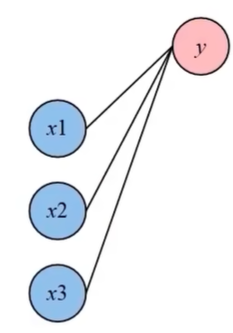
  前向传播：

  ​ 将输入特征通过神经网络逐层计算，最终得到输出特征

  神经元节点的计算过程：

  ​ y = w₁x₁ + w₂x₂ + w₃x₃

  ​ 由于方程是线性的，因此必须在外面套一个非线性的函数σ，称为激活函数

  反向传播：

  ​ 经过前向传播得到预测值后，通过损失函数计算差距，通过调整参数使得损失函数变小

• 测试网络

  使用测试集正向传播来测试准确率

• 使用网络

DNN的实现

查看损失函数、激活函数、层、优化算法等的文档，记得选择自己的版本：http://pytorch.org/docs/1.12/nn.html

批量梯度下降

一次性用 整个训练集 计算梯度，再更新权重

优点：

• 梯度是对整个数据集的精确估计，更新方向稳定。

缺点：

• 数据集大时，计算量大，训练慢
• 占用内存大

import torch
import torch.nn as nn
import  matplotlib.pyplot as plt

class DNN(nn.Module):
    def __init__(self):
        """ 搭建神经网络各层 """
        super(DNN, self).__init__()
        self.net = nn.Sequential(   # 顺序搭建各层
            nn.Linear(3, 5, ), nn.ReLU(),   # 第1层，全连接层，输入3，输出5，ReLU为激活函数
            nn.Linear(5, 5, ), nn.ReLU(),   # 第2层，全连接层
            nn.Linear(5, 5, ), nn.ReLU(),   # 第3层，全连接层
            nn.Linear(5, 3, ), nn.ReLU()    # 第4层，全连接层
        )
    def forward(self, x):
        """ 前向传播 """
        """ 张量会自动计算梯度，不需要反向传播方法 """
        y = self.net(x) # 输入数据
        return y        # 输出数据

# 模拟输入数据集，rand为均匀分布
X1 = torch.rand(10000, 1)
X2 = torch.rand(10000, 1)
X3 = torch.rand(10000, 1)

# 模拟输出特征
Y1 = ( (X1 + X2 + X3) < 1 ).float()
Y2 = ( ((X1 + X2 + X3) > 1) & ((X1 + X2 + X3) < 2) ).float()
Y3 = ( (X1 + X2 + X3) > 2 ).float()

# 整合数据集，把数据放到gpu上
Data = torch.cat([X1, X2, X3, Y1, Y2, Y3], axis = 1)
Data = Data.to('cuda:0')

# 划分训练集和测试集
train_size = int(len(Data) * 0.7)
tes_size = len(Data) - train_size
Data = Data[torch.randperm(Data.size(0)), :]    # 打乱数据集顺序
train_Data = Data[:train_size, :]
test_Data = Data[train_size:, :]

# 创建模型子类
model = DNN().to('cuda:0')

# 查看内部参数
# for name, param in model.named_parameters():
#     print(f"参数:{name}\n形状:{param.shape}\n数值:{param}")

# 选择损失函数
loss_fn = nn.MSELoss()

# 选择学习率与优化算法
learning_rate = 0.01
optimizer = torch.optim.SGD(model.parameters(), lr=learning_rate)


######训练网络

# epochs为每个样本会正反向传播的次数
epochs = 1000
losses = []     # 记录损失函数

# 给训练集划分输入和输出
X = train_Data[:, :3]
Y = train_Data[:, -3:]

for epoch in range(epochs):
    Pred = model(X)     # 一次前向传播
    loss = loss_fn(Pred, Y)     # 计算损失函数
    losses.append(loss.item())  # 记录损失函数的变化
    optimizer.zero_grad()       # 清除上一轮滞留的梯度
    loss.backward()             # 一次反向传播
    optimizer.step()            # 优化内部参数

Fig = plt.figure()
plt.plot(range(epochs), losses)
plt.xlabel('epoch')
plt.ylabel('loss')
plt.show()


##### 测试网络
X = test_Data[:, :3]
Y = test_Data[:, -3:]

with torch.no_grad():   # 测试不需要计算梯度，该局部关闭梯度计算功能
    Pred = model(X)
    Pred[:, torch.argmax(Pred, axis=1)] = 1
    Pred[Pred != 1] = 0
    correct = torch.sum( (Pred == Y).all(1) )
    total = Y.size(0)
    print(f'测试集精准度: {100 * correct / total}%')

保存/导出神经网络

torch.save(model, 'model.pth')

导入神经网络

new_model = torch.load('model.pth')

从csv文件里导入数据

# 导入数据
df = pd.read_csv('Data.csv', index_col=0)   # 从csv导入数据
arr = df.values             # Pandas对象转为NumPy数组
arr = arr.astype(np.float32)# 转为float32类型数组
ts = torch.tensor(arr)      # 数组转为张量
ts = ts.to('cuda')

小批量梯度下降

把训练集划分成若干 小批量（mini-batch），每次只用一个批量计算梯度再更新。

优点：

• 计算效率高，比批量梯度下降快
• 梯度有随机性，能跳出局部最优
• 适合 GPU 并行计算

import numpy as np
import pandas as pd
import torch
from torch.utils.data import Dataset, random_split, DataLoader
import torch.nn as nn
import  matplotlib.pyplot as plt

class DNN(nn.Module):
    def __init__(self):
        """ 搭建神经网络各层 """
        super(DNN, self).__init__()
        self.net = nn.Sequential(   # 顺序搭建各层
            nn.Linear(8, 32, ), nn.Sigmoid(),   # 第1层，全连接层，输入3，输出5，ReLU为激活函数
            nn.Linear(32, 8, ), nn.Sigmoid(),   # 第2层，全连接层
            nn.Linear(8, 4, ), nn.Sigmoid(),   # 第3层，全连接层
            nn.Linear(4, 1, ), nn.Sigmoid()    # 第4层，全连接层
        )
    def forward(self, x):
        """ 前向传播 """
        """ 张量会自动计算梯度，不需要反向传播方法 """
        y = self.net(x) # 输入数据
        return y        # 输出数据

model = DNN().to('cuda')

class MyData(Dataset):
    def __init__(self, filepath):
        df = pd.read_csv(filepath, index_col=0)  # 从csv导入数据
        arr = df.values  # Pandas对象转为NumPy数组
        arr = arr.astype(np.float32)  # 转为float32类型数组
        ts = torch.tensor(arr)  # 数组转为张量
        ts = ts.to('cuda')
        self.X = ts[:, :-1]
        self.Y = ts[:, -1].reshape((-1, 1))
        self.len = ts.shape[0]

    def __getitem__(self, index):
        return self.X[index], self.Y[index]

    def __len__(self):
        return self.len

# 划分训练集和测试集
Data = MyData('Data.csv')
train_size = int(0.7 * len(Data))
test_size = len(Data) - train_size
train_Data, test_Data = random_split(Data, [train_size, test_size])

# 批次加载器
train_loader = DataLoader(dataset=train_Data, batch_size=128, shuffle=True)
test_loader = DataLoader(dataset=test_Data, batch_size=64, shuffle=False)

epochs = 500
losses = []

# 损失函数
loss_fn = nn.BCELoss(reduction='mean')
learning_rate = 0.005
optimizer = torch.optim.Adam(model.parameters(), lr=learning_rate)

for epoch in range(epochs):
    for (x, y) in train_loader:
        Pred = model(x)     # 一次前向传播
        loss = loss_fn(Pred, y)     # 计算损失函数
        losses.append(loss.item())  # 记录损失函数的变化
        optimizer.zero_grad()       # 清除上一轮滞留的梯度
        loss.backward()             # 一次反向传播
        optimizer.step()            # 优化内部参数


Fig = plt.figure()
plt.plot(range(len(losses)), losses)

plt.show()

MNIST数据集

一个0-9数字识别的数据集

import torch
from torch.utils.data import Dataset, random_split, DataLoader
import torch.nn as nn
import  matplotlib.pyplot as plt
from torchvision import transforms  # 图像转换，将数据集转化为张量
from torchvision import datasets    # 下载数据集

# 数据预处理,通常用于处理图像数据集输入神经网络
# ToTensor：将图像的[0, 255]变为[0, 1]
# Normalize(0.1307, 0.3081)：让MNIST 数据集接近正态分布
transform = transforms.Compose([
    transforms.ToTensor(),
    transforms.Normalize(0.1307, 0.3081)
])

# 下载训练集
train_Data = datasets.MNIST(
    root='./dataset/mnist/',
    train=True,
    transform=transform,
    download=True
)

# 下载测试集
test_Data = datasets.MNIST(
    root='./dataset/mnist/',
    train=False,
    transform=transform,
    download=True
)

class DNN(nn.Module):
    def __init__(self):
        """ 搭建神经网络各层 """
        super(DNN, self).__init__()
        self.net = nn.Sequential(
            nn.Flatten(),       #图像铺平成一维
            nn.Linear(784, 512, ), nn.ReLU(),
            nn.Linear(512, 256, ), nn.ReLU(),
            nn.Linear(256, 128, ), nn.ReLU(),
            nn.Linear(128, 64, ), nn.ReLU(),
            nn.Linear(64, 10, ), nn.ReLU(),
        )
    def forward(self, x):
        """ 前向传播 """
        """ 张量会自动计算梯度，不需要反向传播方法 """
        y = self.net(x) # 输入数据
        return y        # 输出数据

model = DNN().to('cuda:0')

train_loader = DataLoader(dataset=train_Data, batch_size=64, shuffle=True)
test_loader = DataLoader(dataset=test_Data, batch_size=64, shuffle=False)

# 设置损失函数和学习率
loss_fn = nn.CrossEntropyLoss()
learning_rate = 0.01
optimizer = torch.optim.SGD(
    model.parameters(),
    lr=learning_rate,
    momentum=0.5    # 是梯度下降算法有了力和惯性
)

epochs = 5
losses = []
for epoch in range(epochs):
    for (x, y) in train_loader:
        x, y = x.to('cuda:0'), y.to('cuda:0')
        Pred = model(x)     # 一次前向传播
        loss = loss_fn(Pred, y)     # 计算损失函数
        losses.append(loss.item())  # 记录损失函数的变化
        optimizer.zero_grad()       # 清除上一轮滞留的梯度
        loss.backward()             # 一次反向传播
        optimizer.step()            # 优化内部参数

Fig = plt.figure()
plt.plot(range(len(losses)), losses)

plt.show()

CNN和DNN的区别

CNN: Convolutional Neural Network，卷积神经网络

特性	DNN（深度神经网络）	CNN（卷积神经网络）
基本单元	全连接层（每个神经元都与前一层所有神经元相连）	卷积层 + 池化层
参数量	参数多（因为全连接）	参数少（卷积核共享权重）
特征提取	人工设计特征，输入通常是向量	自动提取局部特征，适合图像/时序
输入格式	一维向量	二维/三维张量（图像：高×宽×通道）
适用场景	简单分类、回归、推荐系统	图像识别、目标检测、语音识别、NLP（部分场景）

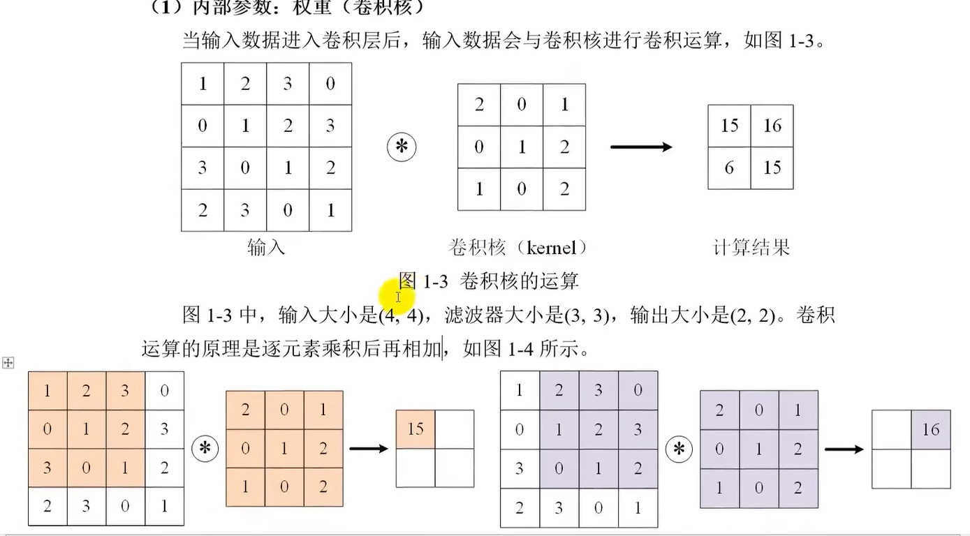
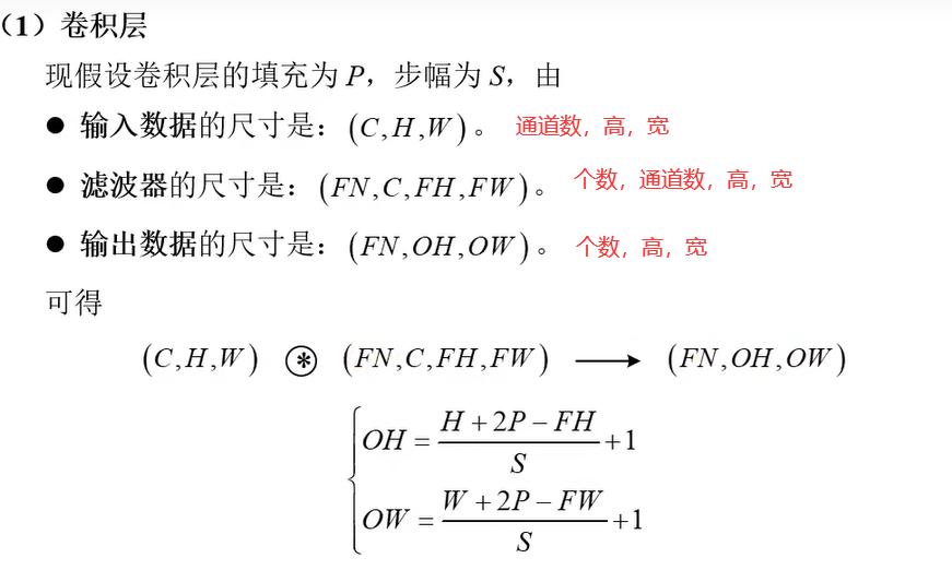
CNN的大致原理

内部参数：卷积核

当输入数据进入卷积层后，会与卷积核（类似DNN的权重）进行卷积运算

当输入数据是二维时被称为卷积核，三维及以上时称为滤波器

内部参数：偏置

将卷积运算结果加上偏置的值

外部参数：填充

为了防止经过多个卷积层后图像越来越小，向图像的周围填充固定的数据（如0）

外部参数：步幅

使用卷积核的位置，每次往右移动1格就是步幅为1

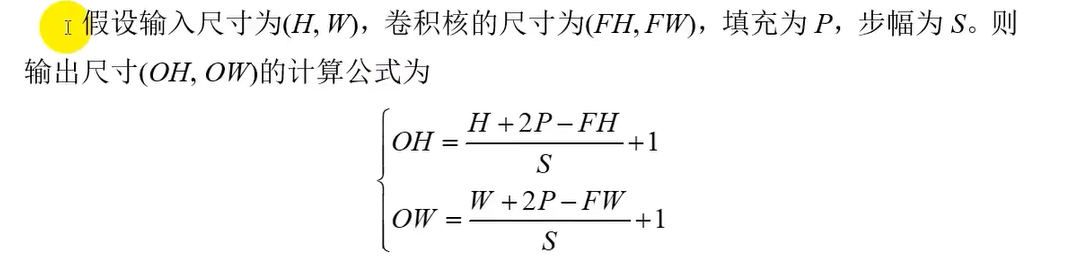
输入和输出尺寸的关系

可通过调节步幅和尺寸来控制某层输出尺寸

多通道输出

让三维的特征多经过几个卷积层，每层都有单独的偏置

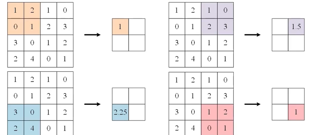
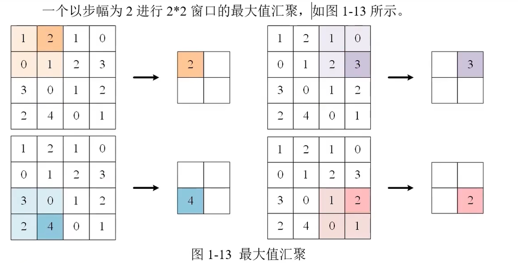
汇聚（池化）

从一个范围内提取一个特征值，不会改变通道数

• 平均汇聚

  

• 最大值汇聚

  

尺寸变换总结

汇聚只要高和宽除以步长就行

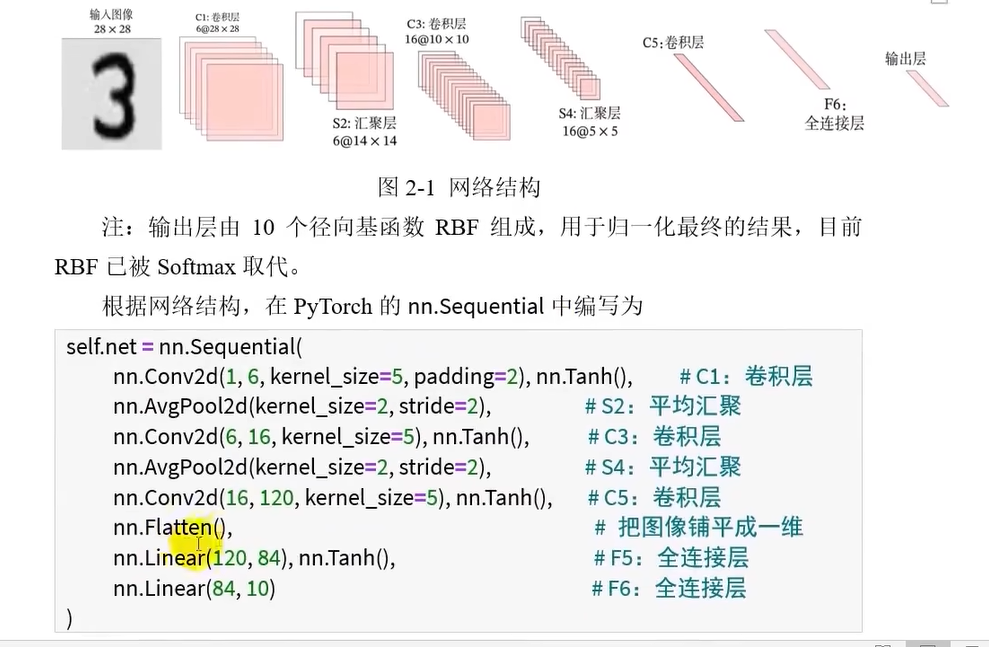
CNN模型

LeNet-5

LeNet-5 是卷积神经网络（CNN）发展史上的一个里程碑模型，1998 年提出，第一个真正成功应用在图像识别上的 CNN 架构，为后来的 AlexNet、VGG、ResNet 奠定了基础

import torch
from torch.utils.data import Dataset, random_split, DataLoader
import torch.nn as nn
import  matplotlib.pyplot as plt
from torchvision import transforms  # 图像转换，将数据集转化为张量
from torchvision import datasets    # 下载数据集

transform = transforms.Compose([
    transforms.ToTensor(),
    transforms.Normalize(0.1307, 0.3081)
])

# 下载训练集
train_Data = datasets.MNIST(
    root='./dataset/mnist/',
    train=True,
    transform=transform,
    download=True
)

# 下载测试集
test_Data = datasets.MNIST(
    root='./dataset/mnist/',
    train=False,
    transform=transform,
    download=True
)

# 批次加载器
train_loader = DataLoader(dataset=train_Data, batch_size=256, shuffle=True)
test_loader = DataLoader(dataset=test_Data, batch_size=256, shuffle=False)

class CNN(nn.Module):
    def __init__(self):
        super().__init__()
        self.net = nn.Sequential(
            nn.Conv2d(1, 6, kernel_size=5, padding=2), nn.Tanh(),   # 卷积层
            nn.AvgPool2d(kernel_size=2, stride=2),          # 平均汇聚
            nn.Conv2d(6, 16, kernel_size=5), nn.Tanh(), # 卷积层
            nn.AvgPool2d(kernel_size=2, stride=2), nn.Tanh(),   # 平均汇聚
            nn.Conv2d(16, 120, kernel_size=5), nn.Tanh(),   # 卷积层
            nn.Flatten(),   # 图像铺平成一维
            nn.Linear(120, 84), nn.Tanh(),  # 全连接层
            nn.Linear(84, 10)   # 全连接层
        )

    def forward(self, x):
        return self.net(x)

# 查看网络结构
# X = torch.rand(size=(1, 1, 28, 28))
# for layer in CNN().net:
#     X = layer(X)
#     print(layer.__class__.__name__, 'output shape: \t', X.shape)

# 创建实例
model = CNN().to('cuda:0')

# 损失函数
loss_fn = nn.CrossEntropyLoss()

# 优化算法
learning_rate = 0.9
optimizer = torch.optim.SGD(
    model.parameters(),
    lr=learning_rate
)

# 训练网络
epochs = 5
loss_list = []

for epoch in range(epochs):
    for (x, y) in train_loader:
        x, y = x.to('cuda:0'), y.to('cuda:0')
        Pred = model(x)
        loss = loss_fn(Pred, y)
        loss_list.append(loss.item())
        optimizer.zero_grad()
        loss.backward()
        optimizer.step()

Fig = plt.figure()
plt.plot(range(len(loss_list)), loss_list)
plt.show()

# 测试网络
correct = 0
total = 0

with torch.no_grad():
    for x, y in test_loader:
        x, y = x.to('cuda:0'), y.to('cuda:0')
        Pred = model(x)
        _, predicted = torch.max(Pred.data, 1)
        correct += torch.sum((predicted == y))
        total += y.size(0)

print(f'精度：{100 * correct / total}%')

AlexNet

AlexNet 是一个经典的 卷积神经网络（CNN）结构，由 Alex Krizhevsky 在 2012 年提出，用于图像分类。它在 ImageNet 图像识别竞赛（ILSVRC 2012）上夺冠，把前一年的错误率从 26% 一下子降到 15% 左右，震惊了整个计算机视觉领域，也标志着 深度学习在视觉任务上的崛起。

GoogLeNet

最特别的地方是 Inception 模块（也叫“Google Inception”），
主要解决 怎么在同一层里兼顾不同大小的卷积核的问题。

ResNet

ResNet，全称 Residual Network（残差网络），是 微软研究院 在 2015 年提出的 CNN 架构。
它在 ImageNet 2015 比赛里直接拿了冠军，把网络层数推到了 152 层，但依然能很好训练，性能远超前辈。

是一种解决深层网络退化问题的 CNN，通过“残差连接”让信息和梯度能顺畅流动，从而能训练几十甚至上百层的网络。